Be SMART and create a portfolio that will beat the market in both theory and practice - The Development and Evaluation of the SMART Investment Model.

Umeå School of Business and Economics

Department of Business Administration

Master Thesis Spring 2006

Supervisor: Åke Gabrielsson

Authors:

Björn Backgård

Fredrik Åkerström

- The Development and Evaluation of the SMART Investment Model -

PREFACE

Before anything else we would like to thank those who made it possible for us to avoid the

sunlight for such a long time, SIX¹ and their database SIX Trust. We would especially like to

thank Henrik Röhs at SIX because without his help this thesis would simply not have been

possible. We would also like to thank our supervisor Åke -Method Man- Gabrielsson for

sharing his great knowledge in the field of scientific methodology and science philosophy and

for pushing us - two pragmatic fools maybe not ideally suited for the academic world -

towards putting more effort into the chapter on methodology.

¹ SIX, http://www.six.se/ (2006-04-29)

ABSTRACT

In this thesis we examine the Swedish stock market to evaluate a trading strategy exploiting

three anomalies known to exist in markets all over the world. The first anomaly is the size

effect meaning that small cap stocks tend to outperform large cap stocks over longer time

periods. The second is the book-to-market (B/P) effect or that firms with high book values

relative to their market value historically have provided greater shareholder returns than firms

with low book values relative to market value. The third anomaly that our model tries to profit

from is the observation that shares having performed well over the last 3 to 12 months

perform better than firms that have performed badly over this time period. We investigate the

presence of these anomalies on the Swedish stock market over the years 1995-2005 and also

try to find out if there are any interrelations between them that can be used in stock selection

and portfolio formation.

Our model for stock selection first divides the available shares into two groups: small cap and

large cap. These two groups are then separated into three subgroups based on their book-to-

market values and these are finally divided into winner and loser portfolios. Each year

between 1995 and 2005 (data included from 1994) we form 12 different portfolios of shares

from the Swedish A-list and compare the returns gained by holding these. All data on size,

book-to-market ratios and momentum as well as returns are collected from the SIX-Trust

database, index returns were obtained from the website of Stockholmsbörsen. Because of

missing data and short periods of listing, we were not able to include all stock from all years

but we managed to include a total of 678 observations of stock data in our sample which

should yield reliable results. The formation of the SMART-model was based on the findings

of many well renowned papers on market anomalies. The way in which we wished to

contribute to the vast amount of anomaly research was to see if the SMART model could

exploit any interrelations between the three anomalies that are part of it, furthermore we

wanted to contribute to the limited amount of research on momentum effects on the Swedish

stock market.

The results of our study were not entirely in line with theory but the SMART-model still

proved to be quite effective. Even though the portfolio expected to perform the best proved

only to be the third best portfolio over the 11 years, it still outperformed the portfolio

expected to be the least effective by more than 20 %. Ranking the portfolios after their

Sharpe-ratios, the predicted winner steps up to a second place with a ratio of .68 compared to

that of - 0,17 for the predicted loser. We also find that that the portfolio formation of the

SMART-Model exploits some interrelationships between the three anomalies: The difference

in return of the portfolios mentioned above is over 20 % while the average difference between

stocks with small and large size, high and low book-to-market and winners and losers is only

just over

4 %. The three anomalies: the size effect, the book-to-market effect and the

momentum effect were also identified to exist in our study, but only B/P was strong enough to

be statistically significant. However, in contrast to what theory predicts, firms with medium

book-to-market values performed worse than those with low ratios. Combining the anomalies

into the SMART-Model proves to be more effective than separately exploiting the anomalies.

This shows that the model can indeed be a useful tool for forming portfolios and that we have

discovered some interesting interrelationships which we suggest further research on.

Index

1 INTRODUCTION

1.1 BACKGROUND

1.2 PROBLEM DISCUSSION

1.3 OBJECTIVE

1.4 DELIMITATIONS

1.5 TARGET AUDIENCE

1.6 DISPOSITION

2 METHODOLOGY

2.1 PRECONCEPTIONS

2.2 SCIENTIFIC IDEALS

2.3 SCIENTIFIC APPROACH

2.4 CONTRIBUTION

2.6 LITERATURE SEARCH

2.6.1 Source criticism

3 THEORY AND THE SMART MODEL

3.1 THEORIES

3.2 MODELS

3.3 THE CAPITAL ASSET PRICING MODEL

3.4 THE FAMA AND FRENCH THREE-FACTOR MODEL

3.5 MARKET EFFICIENCY

3.6 THE SIZE EFFECT

3.6.1 Summary of findings regarding the size effect

3.7 THE MOMENTUM EFFECT

3.7.1 Behavioural explanations for the anomaly

3.7.2 Empirical evidence of the price momentum effect

3.7.3 Summary of empirical findings

3.8 THE ANOMALY RATIO

3.8.1 Summary on the Anomaly Ratio

3.9 INTRODUCTION TO THE SMART MODEL

3.9.1 Motives for selecting the three specific factors Size, Momentum and B/P

3.10 SMART (SIZE-, MOMENTUM- AND ANOMALY RATIO -TECHNIQUE)

3.10.1 SMART METHOD FOR SORTING PORTFOLIOS

3.10.2 OTHER SIMILAR RESEARCH

3.11 RISK MEASURES FOR SMART

3.11.1 Standard deviation

3.11.2 Sharpe ratio

3.11.3 Reasons for selecting the Sharpe ratio

3.11.4 Example of the Sharpe ratio

3.12 HYPOTHESES

4 DATA MANAGEMENT AND TREATMENT

4.1 DATA MANAGEMENT

4.2 POTENTIAL PROBLEMS REGARDING PORTFOLIO CREATION

5 EMPIRICAL EVALUATION OF THE SMART MODEL

5.1 SMART 1995

5.2 SMART 1996

5.3 SMART 1997

5.4 SMART 1998

5.5 SMART 1999

5.6 SMART 2000

5.7 SMART 2001

5.8 SMART 2002

5.9 SMART 2003

5.10 SMART 2004

5.11 SMART 2005

5.12 SMART MEAN RESULTS 1995-2005

5.13 SMART SHARPE RATIO 1995-2005

5.14 CORRELATION ANALYSIS FOR 1995-2005

5.14.1 Correlations calculation with actual-values 1995-2005

6 ANALYSIS

6.1 ANALYSIS OF THE RESULTS

6.1.1 Bringing Sharpe into the picture

6.1.2 Evaluation of interrelations

6.1.3 Findings regarding B/P volatility

7 CONCLUSION

7.1 THE IMPORTANCE OF COMBINATIONS

7.2 OUR OWN SPECULATIONS ABOUT THE REASONS FOR THE ANOMALIES

7.2.1 The Size effect according to us

7.2.2 The B/P effect according to us

7.2.3 The Momentum effect according to us

7.3 CONCLUDING REMARKS

7.4 SUGGESTIONS FOR FURTHER RESEARCH

8 VALIDITY AND RELIABILITY

8.1 RELIABILITY

8.2 VALIDITY

8.3 TRANSFERABILITY

8.4 TESTING FOR SURVIVORSHIP BIAS

8.5 ANALYSIS OF MISSING DATA

9 BIBLIOGRAPHY

9.1 ARTICLES

9.2 INTERNET

APPENDIX A - DIAGRAMS

Figures

Figure 3:1 Diversifiable risk and Systematic risk, p. 9

Figure 3:2 Security Market Line (SML), p. 9

Figure 3:3 Momentum, p. 14

Figure 3:4 SMART method for sorting portfolios, p. 25

Figure 5:1 Total return from starting value of 100 for SMART (all portfolios), L-L-H and AFGX, p. 41

Figure 5:2 Normal QQ plot for factors, p. 42

Figure 6:1 Total return from starting value of 100 for S-H-H, L-L-L, AFGX, p. 46

Figure 6:2 Total return from starting value of 100 for L-L-H, L-L-L, AFGX, p. 58

Tables

Table

3.1 SMART portfolio combinations, p. 24

Table

3.2 Top 20 US funds ranked by the Sharpe ratio, p. 28

Table

5.1 SMART 1995, p. 35

Table

5:2 SMART 1995 Ranking of portfolios, p. 35

Table

5:3 SMART 1995 Mean of main factors, p. 35

Table

5.4 SMART 1996, p. 35

Table

5:5 SMART 1996 Ranking of portfolios, p. 35

Table

5:6 SMART 1996 Mean of main factors, p. 35

Table

5.7 SMART 1997, p. 36

Table

5:8 SMART 1997 Ranking of portfolios, p. 36

Table

5:9 SMART 1997 Mean of main factors, p. 36

Table

5.10 SMART 1998, p. 36

Table

5:11 SMART 1998 Ranking of portfolios, p. 36

Table

5:12 SMART 1998 Mean of main factors, p. 36

Table

5.13 SMART 1999, p. 37

Table

5:14 SMART 1999 Ranking of portfolios, p. 37

Table

5:15 SMART 1999 Mean of main factors, p. 37

Table

5.16 SMART 2000, p. 37

Table

5:17 SMART 2000 Ranking of portfolios, p. 37

Table

5:18 SMART 2000 Mean of main factors, p. 37

Table

5.19 SMART 2001, p. 38

Table

5:20 SMART 2001 Ranking of portfolios, p. 38

Table

5:21 SMART 2001 Mean of main factors, p. 38

Table

5.22 SMART 2002, p. 38

Table

5:23 SMART 2002 Ranking of portfolios, p. 38

Table

5:24 SMART 2002 Mean of main factors, p. 38

Table

5.25 SMART 2003, p. 39

Table

5:26 SMART 2003 Ranking of portfolios, p. 39

Table

5:27 SMART 2003 Mean of main factors, p. 39

Table

5.28 SMART 2004, p. 39

Table

5:29 SMART 2004 Ranking of portfolios, p. 39

Table

5:30 SMART 2004 Mean of main factors, p. 39

Table

5.31 SMART 2005, p. 40

Table

5:32 SMART 2005 Ranking of portfolios, p. 40

Table

5:33 SMART 2005 Mean of main factors, p. 40

Table

5:34 SMART 1995-2005 (average: 14,73, AFGX: 15,56), p. 40

Table

5:35 SMART 1995-2005 Summary for main factors, p. 40

Table

5:36 Standard Deviation, p. 41

Table

5:37 Ranking by Sharpe Ratio, p. 41

Table

5:38 Ranking by Mean Returns, p. 41

Table

5:39 Summary of statistical data, p. 42

Table

5:40 Correlation with actual values, p. 42

Table

6:1 Winning portfolios each year, p. 45

Appendix A

Figure A:1 Total return from starting value of 100 for L-H-H, L-H-L, p. 63

Figure A:2 Total return from starting value of 100 for L-M-H, L-M-L, p. 63

Figure A:3 Total return from starting value of 100 for L-L-H, L-L-L, p.63

Figure A:4 Total return from starting value of 100 for S-H-H, S-H-L, p.64

Figure A:5 Total return from starting value of 100 for S-M-H, S-M-L, p.64

Figure A:6 Total return from starting value of 100 for S-L-H, S-L-L, p.64

Figure A:7 Total return from starting value of 100 for Large, Small and AFGX, p. 65

Figure A:8 Total return from starting value of 100 for B/P High, B/P Medium, B/P Low and AFGX, p. 65

Figure A:9 Total return from starting value of 100 for Momentum High, Momentum Low and AFGX, p. 65

Figure A:10 Total return from starting value of 100 for SMART, L-L-H and AFGX, p. 66

═════════════════════INTRODUCTION═════════════════════

1 INTRODUCTION

In this chapter the reader is introduced to the background of our study. A discussion

will lead forward to a specific problem and a suggestion of a model which will be the

objective to evaluate during this thesis

1.1 Background

In Finance research there has been a long debate whether markets are efficient or not, and if it

is possible to earn abnormal returns by using a special model or strategy. When a variable is

able to predict returns again and again on the stock market it speaks against the Efficient

Market Hypothesis and is therefore called an anomaly. Several well known examples of

anomalies exist; The January effect (stocks have higher returns during this month), The Small

firm effect (small companies generates higher returns than large companies), The P/E effect

(Low P/E stocks have higher returns than High P/E stocks), Neglected firm effect (the market

sooner or later discovers firms that are in good standing but have been overlooked by the

market), Book-to-Market effect (stocks with a high ratio for B/M or B/P have abnormally high

returns).² Some argue that several of these are actually related to each other and that they

more or less overlap one or more of the others to some degree, or even absorbs another like

Reinganum claimed Size did to the P/E effect.

Doing research on market anomalies is not just about finding ways to make abnormal profits,

it also serves as a process to help eliminating them and making financial markets more

efficient. And the more rational financial markets behave, the more predictable they will be,

and the more predictable they are the less risky it will be for individuals to place their funds in

stocks. If markets are irrational and unpredictable shares will at different times be either

under- or overvalued which means that some individuals placing their savings in stocks will

make great profits while others will suffer losses. When the outcome of investing in the stock

market seems uncertain or even random, investors will demand higher returns, pushing prices

downwards. The outcomes of all factors affecting share prices of course cannot be fully

predicted, but market anomalies make prices behave even more volatile. The rational for the

existence of financial markets is to allow individuals to allocate their funds over time by

saving or borrowing in order to maximize their utility. When the prices of stocks are lower

than they would be than in a world with efficient markets, it means that individuals will be

pushing forward more of their life time consumption than necessary which means that their

total wealth seen over a lifetime, will be lowered. Therefore, it can be concluded that market

anomalies are bad for individuals and for society as a whole. By shedding light on the

irrationalities present in stock markets, they should eventually go away. This way resource

allocation will work more efficient and individuals will be better off.

In our thesis we will concentrate on three of the above mentioned anomalies. Many research

articles give evidence that simple trading strategies based on anomalies can actually be used

to earn abnormal returns. Firm Size and the B/P ratio can be used to earn higher returns than

one should expect based on CAPM. These anomalies are incoherent with the Efficient Market

² Bodie, Z. Kane, A. Marcus, A. Investments - 6^th International Edition (New York: McGraw-Hill/Irwin, 2005),

p. 389-396

═════════════════════INTRODUCTION═════════════════════

Hypothesis (EMH). A common strategy in practise is also to use Momentum Based Strategy

(MBS) and take advantage of trends in the market. None of these should be possible to exploit

if the markets were fully efficient, any abnormal profit opportunities would be arbitraged

away and disappear with time. However this does not seem to be the case for the three factors

that are the foundation of the model we are going to test in this thesis. Their effects does not

seem to fade away with time. We are going to study if the combination of these anomalies

would create even larger abnormal returns, or if they somehow level out each other and are

only useful if used one at a time? It will be done by testing a model that will reveal if any

combination of these factors are especially interesting in the eyes of an investor. The name we

came up with for this model was SMART, Size- Momentum- and Anomaly Ratio Technique.

The name SMART means the same thing in both Swedish and English. If we play around

with the word and spell it backwards something amusing happens, “TRAMS”, which in

Swedish means “RUBBISH”. Let’s just hope we don’t get the latter result when testing our

model..

In the research articles we based the theories on the Size and B/P effects are often studied

simultaneously, and usually in attempts to test the CAPM model and Beta. To initiate the

reader to the subject we present the textbook description:

“The tendency for stocks of firms with high ratios of Book-to-Market value to generate abnormal returns.”³

“Fama and French found that after controlling for the size and book-to-market effects, beta seemed to have no

power to explain average security returns. This finding is an important challenge to the notion of rational

markets, since it seems to imply that a factor that should affect returns – systematic risk – seems not to matter,

while a factor that should not matter – the Book-to-Market ratio – seems capable of predicting future returns.”⁴

When reading Fama & French and others, we often see the words Cross-section analysis and

Time-series analysis. This could be a good time to clarify these for the reader. Cross-section

data are a collections of data like prices on stocks or market values, at a specific point in time.

We will study the values of Size, B/P and Momentum at the end of each year and therefore

this study could be characterized as a Cross-sectional study. Time-series presents changes

over time of one particular variable, for example the price of one stock over time.⁵ Since a

Cross-sectional study like the one we have done, with historical values and ratios, involves

many problems with gathering data and getting the right data it’s not possible to completely

simulate historical situations on the market. There will be biases in testing and missing data

for stocks etc that we need to discuss later on. But we are quite sure that we have sufficient

data for the SMART model to be tested properly. For the period 1995-2005 we have gathered

data on nearly 140 stocks that are or have been located on the Swedish stock exchange, more

specifically on the A-list. For different reasons, that will be discussed more later, the number

is reduced to between 50-100 each year that will actually be included in the portfolio

formation that will be an essential part of testing the SMART model. There are more stocks

on the A-list during the first half of the studied period than on the second. A total number of

132 portfolios of stocks will be combined during 11 years (1995-2005) which in other words

means a lot of time in front of the computer screen rather than in the sunlight.

³ Bodie, Z. Kane, A. Marcus, A. Investments - 6^th International Edition (New York: McGraw-Hill/Irwin, 2005),

p. 1048

⁴ Bodie, Z. Kane, A. Marcus, A. Investments - 6^th International Edition (New York: McGraw-Hill/Irwin, 2005),

p. 392

⁵ Watsham, T. J. & Parramore, K. Quantitative Methods in Finance. (Oxford: Thomson Learning), p. 42

═════════════════════INTRODUCTION═════════════════════

1.2 Problem discussion

Different articles proposed several explanations for the Size and B/P effects but a majority of

them agreed that these effects are real and existed both in USA and internationally.

Furthermore there is much evidence that the Momentum Based Strategy (MBS) consistently

produce abnormal returns. The foundation for MBS is that the performance of stocks follows

trends in the short run. Therefore you could “ride the wave” and buy winners in an upward

trend, and without much analysis get good returns during shorter holding periods. Our idea is

to combine Size, B/P and MBS into one model and test it on the Swedish stock market to see

if this would produce abnormal returns comparable to the individual effects of the factors, or

if we discover that combinations of them actually reduce or enhance the returns. Would it be

possible to get considerably higher returns than the market index by combining anomalies?

Could it have been possible to earn very high average return on the Swedish market between

1995-2005, by using only the values of three anomalies as a foundation for an investment

strategy? This should not be possible according to EMH since the effects should disappear

when discovered. This will be the main scientific problem area we will seek an answer to. For

this purpose we developed SMART, which is a model that specifies all possible combinations

of Large/Small Size - High/Medium/Low Book-to-Market - High/Low Momentum. By this

approach we will be able to detect any superior permutations based on the historical data.

1.3 Objective

The objective of this thesis is to evaluate if it is possible to earn abnormal risk-adjusted

average returns by using one or more of the combinations suggested by our SMART model.

1.4 Delimitations

We will study the stocks listed on the A-list on the Swedish stock exchange during the period

1995-2005. Looking at a longer time span would normally increase the accuracy of the

results, but there are several reasons for limiting the sample period to the period that we have

chosen to work with. First of all, the data for the years preceding

1995 are not as

comprehensive as those for 1995 and forward. Another reason to start at this year is that the

early nineties were characterised by changes in tax regulations, in monetary regulations and

by a sharp recession. We envisioned that all this turbulence could bring to much noise into the

dataset, and as the reason for including more observations would be to increase the reliability

this could very well be counterproductive. The momentum effect has also already been

documented by Rouwenhorst up until 1995 on the Swedish stock market which means that we

would not make any contribution to this area of research by including years prior to this date.

The results derived from the model will be valid for this period, but may or may not be

applicable during other time periods or in other countries.

There are more known anomalies than those we investigate in this thesis. The reason we

chose to focus on the momentum, size and book-to-market effects will be described in detail

in chapter

3.9.1 but in sort it was mainly because they are the most documented and

researched anomalies that can be combined into a portfolio strategy. The Small firm January

effect can not be used when investing with a one year holding period and the P/E effect - as

will be seen in chapter 3.6 - has been shown to disappear when controlling for the Size effect.

═════════════════════INTRODUCTION═════════════════════

1.5 Target audience

Students and professionals interested in finance and investment, especially in ratio analysis

and portfolio management, but also economists and other audiences interested in efficient

markets and behavioural biases.

1.6 Disposition

This thesis will start with a description of the methodology used to investigate the

components of the SMART model. Then we continue with a theoretical orientation and a

historical research overview of the field. This will build a foundation for the development of

the SMART model. We will then present the empirical findings and then comment on these in

the analysis and link it with the theories. Finally we draw conclusions and test if the

hypotheses holds or not and which implications this may have. The disposition of this thesis

could be represented as a drop-down list of topics that will illustrate their position in the

thesis, as well as preparing the reader for what to come.

Method -> Orientation -> Development -> Empirical findings -> Logical conclusions

Introduction

SMART

Analysis

Theories

Methodology

1995-2005

Conclusions

Hypotheses and models

Mean results

Recommendations

Efficient Market Hypothesis

Rankings

Size effect

Momentum effect

Anomaly ratio

Risk measures

Treatment of data

════════════════════METHODOLOGY═════════════════════

2 METHODOLOGY

In this chapter we present the various method choices we have made in an attempt to

succeed in answering the objective of this thesis. We will also motivate these

selections. We start with a statement of preconception and describe the approach we

have chosen, and how we have conducted this study with gathering of information

and analysis of data.

2.1 Preconceptions

Past studies, interests and experiences influences how we act and react to the environment

around us. Therefore it could be interesting for the reader to know a little about our

background. Both Björn and Fredrik are, at the time of writing this thesis, in the end of our

studies at the master year in Finance & Control. Among others, the master’s program includes

the courses Investments, Corporate finance and Analysis of financial data during which

market efficiency and anomalies have been examined. Björn has also taken a course in

financial economics on a bachelor level which also touched these areas. Fredrik has in

addition studied various business courses on the bachelor level abroad at APU in Cambridge

(England). Another thing we have in common except our current studies, is our high school

background from natural science studies, a field which’s methodologies we have used in this

thesis. We have not worked in the field of finance but Fredrik has stock investment as a hobby

(and is a firm believer in Momentum Based Strategy) and both of us are interested in working

within the field of finance in the future. This should however not undermine our ability to

value and analyse the results objectively, rather the opposite. Since we are very interested in

this field and the ability to use the results from this thesis for our own gains, our motivation

for producing highly accurate data is particularly strong. Finally, it should be mentioned that

neither of us believes in the absence of behavioural biases in securities markets, we simply do

not believe in the existence of the homo economicus.

2.2 Scientific ideals

There are several ideals or schools in the scientific community, but since this is a thesis in

finance and not scientific philosophy we limit ourselves to justify the choice between the two

main ideals usually discussed. This thesis is positivistic in nature. Positivistic derives from the

Latin word positivus and means determined or known. The term is closely related to natural

science. When you follow this you value secure, objective and measurable knowledge.⁶ We

intend to test, reject and verify theories with the aid of historical data in an objective manner,

which is why the positivistic approach will suit this thesis well. The hermeneutic school is

concerned with interpretation where you use you own preconceptions as a subjective tool for

understanding a problem that can’t be quantified or reduced easily to testable hypotheses or

figures. Since we want to avoid subjective biases this method will not be appropriate for this

kind of study. Furthermore the very essence of the raw information we use in our study is

simply numerical representations of reality from the beginning, without much need for

translation or interpretation to understand what it represents. With that said and done we can

start our journey to the more interesting parts, at least from the investors standpoint, that is.

⁶ Franke-Wikberg, S. Vetandets Vägar (The Ways of Knowledge), (Lund: Studentlitteratur, 1994),

p. 323

════════════════════METHODOLOGY═════════════════════

2.3 Scientific approach

In scientific research you usually distinguish between the traditional (quantitative) and the

qualitative method. We will collect and analyse quantitative data and therefore the

quantitative method is the obvious choice. In an argumentation that uses deduction you go

from the general to the specific, when using induction you go in the opposite direction from

the specific to the general.⁷ In other words we will in this thesis move from theory mainly

based on the American environment to the empirical part based on the Swedish environment,

to see how well the theory applies to the Swedish stock market. Furthermore we will test

hypotheses based on the theoretical foundation which is why a deductive approach is more

appropriate for us than an inductive, where you use empirical findings to build a theory. We

already have a theory and a model based on that theory we want to test and therefore the

deductive approach comes naturally.

2.4 Contribution

The empirical part of this thesis will concentrate on the Swedish stock market, or more

specifically on the A-list, where the large and frequent traded companies are listed. Thy

theoretical foundation will be largely influenced by American articles and research, simply

because there is an abundant number of articles concerned with that market and even narrow

subjects usually have relatively much information to build on.

There is much less research on the subject of this thesis done on the Swedish stock market

than on American financial markets. Therefore we will contribute to the field of research by

comparing how accurate and transferable the American research is to the Swedish market on

this particular topic. This thesis will especially expand the knowledge in the way market

anomalies interact, and the focus lies on the Size effect, Momentum and Book-to-Market

(B/P) ratio. As we have not found any research on the momentum effect on the Swedish stock

market subsequent to 1995, we believe that we will make an important contribution in this

area. In general terms our intention is to contribute with knowledge regarding investment

strategy. Our aim is to produce practical knowledge that can be applied in reality for both

private and professional investors.

2.6 Literature search

There is a vast amount of articles produced that are related to the research topic of this thesis

in one way or another. Among the first articles we read were the ones of Penman and Fama &

French, citations from these then led us to a large number of other articles that could have

potential to be included in the thesis. These articles also had a lot of interesting references and

together with the articles found through searching with Google, Business Source Premier,

Lund University Dissertations Abstracts, etc, the problem was not to find enough relevant

articles but to narrow it down and to know which ones that were most important to include.

When searching databases and the web, the keywords we used predominantly were of course

related to the three anomalies like “firm size effects”, “anomalies” “B/M”, “B/P”, “book to

market”, “price to book”, “momentum”, "small firm effect", "abnormal returns", "momentum

⁷ Sellstedt, B. Metodologi för Företagsekonomer - Ett Försök till Positionsbestämning (Methodology for

Business Administrators - An Attempt to Take a Stand), http://swoba.hhs.se/hastba/papers/hastba2002_007.pdf,

p. 64 (2006-04-18)

════════════════════METHODOLOGY═════════════════════

investment", "portfolio strategy", "market efficiency" as well as searching for the exact

authors or articles mentioned repeatedly in other articles. Relatively early we found a great

page at Duke University (The Fuqua School of Business, Top10 ranked in USA) which had

references to high quality research articles that could be relevant for our study. They had a

special page for “PhD Seminar in Empirical Accounting Research” where several of the most

important articles used in this thesis can be found and downloaded.⁸ This enabled us to gain a

better focus on relevant articles. We also found a paper called “A Price To Book Model Of

Stock Prices”⁹ which had a brilliant overview of the research progress in this area that also

mentioned many of the articles found on the Duke University page. This should ensure that

our theories are based on the most respected articles in the field.

2.6.1 Source criticism

As stated above, we have tried to use articles already recommended by well-known authors.

While doing this we also found out that many articles were mentioned repeatedly in other

articles. This cross referencing gave us an idea of which articles were most respected and used

in the academic research, therefore we have based our theoretical chapter heavily on those

articles. Almost all of the articles used for this thesis have been published in financial journals

which should serve as a certification for their reliability. This combined with the use of recent

articles and our aim to always use the primary source when possible is according to us a good

quality ensuring procedure. There is always the risk of misinterpretation and personal bias

when collecting information, especially from advanced articles, but since we have used many

sources and read several articles and their interpretations of the main research work, we

should have eliminated this error to a great extent.

⁸ Duke University, PhD Seminar in Empirical Accounting

Research,http://faculty.fuqua.duke.edu/~jfrancis/PhD%20Seminar/outline.htm

⁹ Branch, B. Sharma, A. Gale, B. Chichirau, C. Proy, J. (2005). A Price To Book Model Of Stock Prices,

University of Massachusetts, http://www.westga.edu/~bquest/2005/model.pdf

══════════════THEORY AND THE SMART MODEL═══════════════

3 THEORY AND THE SMART MODEL

In this part we will discuss the theories and controversies that leads forward to the

SMART investment model and finally the hypotheses of this thesis

3.1 Theories

A theory is a collection of related concepts or definitions with the purpose to explain, interpret

or predict something. The key difference between a theory and a hypothesis is that theories

are more complex and abstract in nature. Theories are tools that we can use to orient

ourselves.¹⁰

3.2 Models

It's not always easy to determine what is a model and what is a theory. One could say that

Models are representations of something while a Theory is an intention to explain that

something. A theory can use a model to explain a phenomenon. Sometimes a problem can

arise that is related to a model's mathematical representation. The model could give a result

that is only valid within two boundaries.¹¹

This is a typical problem discussed when testing the CAPM model. It does not appear to be

valid in the extremes, just like returns are not normally distributed in the extremes, and hence

the normal distribution, and standard statistical tests based on it, can not be used when

examining returns. Investment strategies involving Size, Momentum, and Book-to-Market

appears to be more successful than they should be according to the CAPM, and a common

explanation is that the model’s mathematical representation have problems and therefore can

not make accurate predictions when these anomalies are used in investment strategies, and

therefore it appears like these strategies produce abnormal returns. We will try to use this to

find an investment strategy that consistently produces higher returns than we should expect.

This thesis will investigate anomalies that the CAPM don't predict well.

3.3 The Capital Asset Pricing Model

The CAPM is a famous model that states that returns should be related, or more correct,

proportional to systematic risk. In our opinion CAPM is a fairly good tool, but we do not

believe it is very useful for special cases like the anomalies that our SMART model resides

on. It is nevertheless important to understand the basic concepts of it because many of the

theories and arguments in this thesis will be linked to the CAPM model.

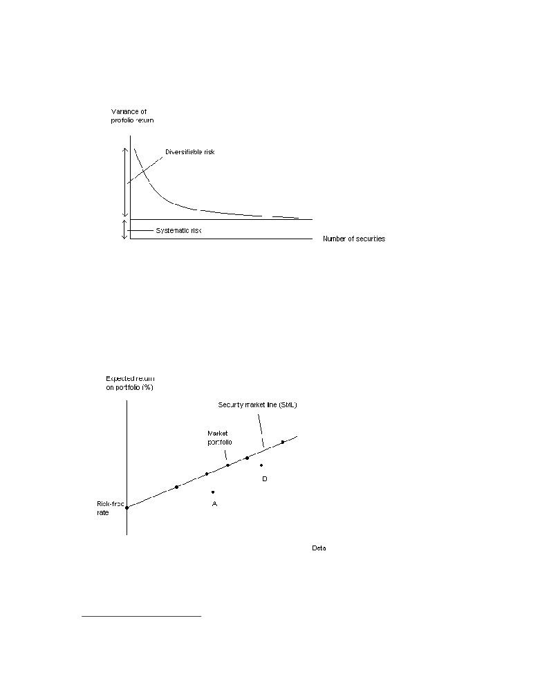
According to the CAPM, the risk of holding securities can be separated into two types:

Diversifiable risk and systematic risk. By forming portfolios, any firm-specific risks can be

effectively eliminated. According to the CAPM, because it can be diversified, exposure to

firm-specific risk does not require a risk-premium. Systematic risk, which measures the extent

¹⁰ Sellstedt, B. Metodologi för Företagsekonomer

- Ett Försök till Positionsbestämning

(Methodology for

Business Administrators

- An Attempt to Take a Stand), SSE/EFI Working Paper Series in Business

Administration No 2002:7, Stockholm School of Economics.

URL: http://swoba.hhs.se/hastba/papers/hastba2002_007.pdf, p. 70 (2006-04-18)

¹¹ Op. Cit

══════════════THEORY AND THE SMART MODEL═══════════════

to which security returns are correlated with market return, on the other hand do justify a risk

premium because it can not be eliminated.¹²

Figure 3.1 Diversifiable risk and Systematic risk.

Important assumptions behind the CAPM are the existences of a market portfolio and of risk-

free borrowing and lending. The market portfolio consists of value-weighted portions of all

securities and will by market mechanisms - where prices adjust to levels where all securities

have the right expected return -become the optimal portfolio to hold. Because the market

portfolio can be combined with risk-free borrowing and lending, a security must lie on the

SML. Portfolios A and B, which are situated below the SML can both be dominated by a

combination of holding the Market portfolio and risk-free borrowing or lending.

Figure 3.2 Security Market Line (SML).

The expected return of a security is by the CAPM expressed by the following formula:

Ri = Rf + βi x (Rm - Rf)

¹² Bodie, Kane, Marcus, Investments - 6^th International Edition (New York: McGraw-Hill/Irwin, 2005), pp. 224,

282.

══════════════THEORY AND THE SMART MODEL═══════════════

Where the only source of risk that is being compensated for in the form of higher expected

return is covariance with the market.¹³

Empirical tests of the CAPM shows that beta, or covariance with the market, is actually not

the only source of risk that carries a risk-premium. Regressions of the form:

Ri - Rf = γ0 + γ1βi + γ2σ²(ei)

Where the hypothesis is that, γ0 and γ2, the intercept term and the coefficient for firm specific

risk, are both equal to zero, which means that all variability in return should be explained by

beta. The tests however show that in reality, the intercept is significantly positive and the

slope pf the SML is too flat for the CAPM to be valid.¹⁴

3.4 The Fama and French Three-Factor Model

The Fama and French three factor model is a regression model with three variables (multiple

regression) often discussed in the theoretical research in the field of finance related to this

thesis. We therefore present it here as a support for the reader. It is not necessary to fully

understand this to be able to interpret the results, but it may be useful for interested readers

that desire to get an in-depth understanding of the debate and controversies around the topic.

For us as authors, we felt obliged to study this in more detail to understand what exactly many

of the articles were trying to convey.

In empirical tests, it has been noted that on average, small firms tend to outperform large

firms and that firms with a high Book-to-Market ratio tend to outperform firms with a low

such ratios. Fama and French argued that these two factors may capture sensitivity to risk

factors in the macro economy and constructed a new model intended to predict security

returns.¹⁵ Apart from the market return, which the CAPM is singly based on, Fama and

French included two additional factors namely the SMB and the HML.

The SMB factor, which measures the difference in return between the stocks of companies

with small and large market capitalization, is calculated by subtracting from the return on

small companies, the return on large ones. Similar to the way in which the risk-free rate is

subtracted from the market rate in the CAPM. The HML factor, or the difference in historic

returns of firms with high Book-to-Market value and firms with low value, is calculated by

subtracting from the return one third of the companies with the highest values, the return on

the companies with the lowest values. The model has the following form:

E(Ri) - rf = ai + bi[E(Rm) - Rf] + siE(SMB) + hiE(HML)

Where (E) stand for expected. Regressions ran over the years 1929 to 1997 and the Three-

factor model showed that all of the coefficients were significant, with R-square statistics all

exceeding 0.91.¹⁶ Further evidence on these factors and some deeper discussion will be

provided in succeeding chapters.

¹³ Bodie, Kane, Marcus, Investments - 6^th International Edition (New York: McGraw-Hill/Irwin, 2005), pp. 282-

293

¹⁴ Op. Cit, p. 418

¹⁵ Op. Cit, p 360

¹⁶ Bodie, Kane, Marcus, Investments - 6^th International Edition (New York: McGraw-Hill/Irwin, 2005), p 429-

430

══════════════THEORY AND THE SMART MODEL═══════════════

3.5 Market efficiency

It is absolutely essential to know and understand the basic concepts behind the Efficient

Market Hypothesis and it’s implications for investment strategy to be able to analyse our

thesis. Here we will only provide a brief overview of the theory. For the interested reader a

vast amount of information is available on the topic with just a few clicks on the mouse so to

speak. Furthermore, we also believe that the readers interested in this thesis are already quite

familiar with the Efficient Market Hypothesis. Even so, it is always good to refresh the

memory.

In a truly efficient market, the prices of securities traded in that market will at all times equal

their true investment values. Because of this, no investor, no matter how skilled he or she is,

and no investment strategy, no matter how sophisticated, will be able to beat the market. A

typical schoolbook definition of the concept is given by Sharpe, Alexander and Bailey in their

book Investments:

A market is efficient with respect to a particular set of information if it is impossible to make

abnormal profits (other than by chance) by using this set of information to formulate buying

and selling decisions.¹⁷

With this definition, all tests of market anomalies are seen as tests of market efficiency,

because in an efficient market no anomalies should exist. At least not to a degree where

abnormal risk-adjusted profits can be made by implementing a strategy exploiting market

anomalies. For example, already in 1981, Banz showed that the expected return was higher

for firms with small market capitalisation than for firms with large market capitalisation.¹⁸

This does not however prove that markets are inefficient, because the size of a company may

be correlated with some other source of risk, causing investors to demand higher profits to

adjust for higher risk when investing in small cap firms.

Market efficiency is commonly described in three forms¹⁹:

1. Weak efficiency, meaning that abnormal profits can not be made using information

about historic prices. This means that technical analysis is ineffective in predicting

returns, which in turn entails that momentum investing, a strategy we will describe

later on in the theoretical framework and finally test empirically, will not be effective.

2. Semi-strong efficiency, under which it will not be possible to make abnormal profits

by using publicly available information about companies. This implies that the size-

effect and the Book-to-Market anomaly should either be non-existing or that the

market capitalisation and Book-to-Market ratios carry some information about risk.

We will later go into these anomalies in detail.

3. Strong efficiency means that share prices at all times reflects all public and private

information.

¹⁷ Sharpe, F. Alexander, G and Bailey, V. (1999). Investments, p. 93

¹⁸ Fama, E.F. & French, K.R. The Cross-Section of Expected Stock Returns

(The Journal of Finance, Vol. 47 No 2 June 1992), p. 427

¹⁹ Sharpe, F. Alexander, G and Bailey, V. (1999). Investments, p. 93

══════════════THEORY AND THE SMART MODEL═══════════════

3.6 The Size effect

It’s been well documented in many research articles that a firm’s size has a siqnificant effect

on the stock returns. Small firms generally generate higher shareholder returns than big

companies. Why this is so, has for a long time been a topic of debate in the academic world,

and some even question that the effect exists as it has not always been found to be significant.

There are actually some indications that the small firm effect might not be valid for the

Swedish stock market (or at least be less pronounced), still, the authors of this thesis are rather

convinced by our own “non-statistically” observations that this is the case. As an example we

have seen that the small company funds on the Swedish market (and internationally) are

usually the best performers over longer time periods. This is of course, at least before writing

this thesis, mainly based on our own limited experience, and not scientific research. Anyway,

we will now present the academic view on this topic.

One common explanation for this is that these firms carry a risk premium which investors are

compensated for by higher returns.²⁰ This is not a new discovery. Reinganum documented

empirical anomalies in 1981 which suggested that either the capital asset pricing model

(CAPM) is misspecified, or that capital markets are inefficient. Portfolios based on firm size

or earnings/price (E/P) ratios produced average returns systematically different from what

CAPM predicted. Reinganum also noticed that the effect was not temporary but remained at

least two years into the future. He state that in his opinion the result reduces the probability of

the size effect being generated by a market inefficiency. Based on the study he did he believes

the equilibrium pricing model is wrongly specified rather than that the market is inefficient.

We agree with the conclusion that the equilibrium pricing model being invalid at least in the

extremes, but don’t agree that markets are efficient. The data also revealed that the E/P effect

did not appear when returns were controlled for the size effect. The firm size effect largely

absorbs the E/P effect. Both of these anomalies exists when studied separately, but they seem

to be related to the same set of missing factors. Reinganum therefore conclude that these

factors are probably more closely linked with the firm size than the E/P ratio.²¹

Accoring to Reinganum two researchers, Leong & Zaima, reported in 1991 that studies have

found that the firm size, measuered as the total market value of equity, is negatively related to

excess returns. In other words big companies generate lower shareholder returns than small

companies. In their own studie they also concluded that the portfolio with the smalles market

value (MV) consistently outperformed the large market value portfolio. The result was

consistent with earlier studies.²² Usually the studies find that there is no big difference in

returns between medium and large firms, but for small firms there is a strong effect. However

Leong & Zaima could not find evidence of a small firm effect on the OTC list (where the

much smaller firms are located). This indicates that the size effect may only apply to the small

companies on the large company lists. On the Swedish stock market this would mean that we

should only expect to find the small firm effect on the A-list but not on the O-list, if the

²⁰ Drew, M. E. Veeraraghavan, M. Beta, Firm size, Book-to-Market equity and Stock Returns ( Journal of the

Asia Pasific Economy, Vol. 8 No 3 October 2003), p. 376

²¹ Reinganum, M. R. Misspecification of Capital Asset Pricing - Empirical Anomalies Based on Earnings' Yields

and Market Values (Journal of Financial Economics, Vol. 9 No 1 March 1981), p. 19

²² See Banz (1981), Reinganum (1981, 1983) and Brown, Kleidon and Marsh (1983) for NYSE-AMEX stocks.

══════════════THEORY AND THE SMART MODEL═══════════════

results could be transfered to the Swedish stock exchange.²³ Many other researchers also

confirms the existence of the size effect to this day.²⁴

3.6.1 Summary of findings regarding the size effect

There is some discussion on the existence of a Size anomaly. Without doubt there is as Size

effect, but whether this is really an anomaly or if the effect arises because of justifiable risk

premiums has not been fully established. The CAPM cannot explain the excess return on

small firm shares, but this model has been rejected by the majority of the community of

financial researchers. The Size effect has been shown to be closely connected to the P/E effect

and there is some evidence saying that the differences in return only exist between the really

large companies and smaller ones.

3.7 The Momentum effect

Pick the winners and throw away the losers. That is the basic idea of momentum investing.

More exactly, momentum investing exploits the market anomaly that shares having performed

the best over the last 3 to 12 months, on average will outperform index for the upcoming

months.

This anomaly was first discovered by the academic world in 1993 by Jegadeesh and Titman

and the existence of it has thereafter been confirmed in several independent studies using

datasets from both developed and emerging markets.²⁵ A survey of mutual fund investors in

1995 indicated that 77 percent of US mutual funds used momentum as a stock selection

criteria, it shows that momentum investing more than just a theoretical model.²⁶ One very

interesting aspect of the momentum effect is that it is reversed when looking at longer time

periods. That is, the winners over the past three to five years tend give less return than index

over the subsequent three to five years while the stocks having performed the worst over the

corresponding time period tend to give the best subsequent return. It appears as if the market

initially under reacts to good news but over some time overreacts and eventually come to its

senses.²⁷

²³ Leong, K. K. & Zaima, J. K. Further Evidence of the Small Firm Effect: A Comparison of the NYSE-AMEX

and OTC Stocks (Journal of Business Finance & Accounting, Vol. 18 No 1 January 1991), p. 117-124

²⁴ See Fama & French (1992), Jensen, Johnson, and Mercer (1997), Maroney & Protopapadakis (1999). Bleiser

(2003), and Carlson, Fisher and Giammarino (2004) to mention a few.

²⁵ Bird, R. Whitaker, J. The Performance of Value and Momentum Investment Portfolios: Recent Experience in

the Major European Markets (Journal of Asset Management, Vol. 4 No 4 December 2003), p. 223

²⁶ Taffler, R. Discussion of the Profitability of Momentum Investing (Journal of Business Finance & Accounting,

Vol. 26 No 9/10, Nov/Dec 1999), p. 1093

²⁷ Daniel, K. Hirshleifer, D. Subrahmanyam, A. Investor Psychology and Security Market Under- and

Overreaction (The Journal of Finance Vol. LIIII No. 6 December 1998), pp. 1839-1840

══════════════THEORY AND THE SMART MODEL═══════════════

Figure 3.3 Momentum - In the figure, there is an initial under reaction followed by an overreaction and

finally a mean reversal. It can be compared to the response of an efficient market.

3.7.1 Behavioural explanations for the anomaly

Several behavioural explanations for the long term overreaction and the short term

underreaction have been provided since the discovery of the market anomaly. Barberis,

Shleifer and Vishny developed a model where investment decisions are characterised either

by representative heuristic or conservatism. When decisions are characterised by the former,

it means that investors put to much weight on recent data and ignore the more complete

statistical evidence on stock types. This leads investors to overreact to new data. When

characterised by the latter, it means that investors are slow to update their models in the face

of new evidence, this leads them to underreact to new data. In the model, at a given time,

predominant view will either be that earnings are mean-reverting, or that they are trending.

Normally, investors will believe earnings to be mean reverting but their opinion may switch to

thinking that earnings are trending after a string of either positive or negative announcements.

When they switch from being conservative to becoming representative heuristic, investors

will overreact to earnings shocks as they expect subsequent earnings shocks to point in the

same direction as they now believe them to be trending. When a positive string of earnings

announcements has occurred, investors will eventually react less to additionally positive

announcements than to negative such. The reason is that the positive news are already more or

less expected and taken into account. Because positive and negative shocks in reality are

equally likely, the result of this is that the returns on average will be negative for the coming

time period. This causes returns to be mean-reverting. On the other hand, when the belief is

that earnings are mean reverting holds, investors will react less strongly to news pointing in

the opposite direction of previous news than to news pointing in the same direction. This way

the reaction to either positive or negative news will be delayed and a momentum effect will

come about.²⁸

Daniel, Hirshleifer, and Subrahmanyam developed a model in 1998 with two types of

investors: informed and uninformed, where the former is the one that decides prices and the

latter follow his actions. The informed investors suffer from overconfidence and variations in

²⁸ Liu, W. Strong, N. Xu, X. The Profitability of Momentum investing

(Journal of Business Finance &

Accounting, Vol. 26 No 9/10, November/December 1999), p. 1047

══════════════THEORY AND THE SMART MODEL═══════════════

confidence arising from biased self-attribution. Daniel, Hirshleifer, and Subrahmanyam

describe an overconfident investor as one who overestimates his or her ability to generate

information and ability to interpret data that others neglect, which leads to overconfidence

about the precision of personal information but not about publicly available information. In

the case when subsequent public information confirms the forecast based on private

information, this will boost the confidence of the investor about his forecasting ability, and

likely cause a further overreaction to the preceding private signal . In the opposite case, when

subsequent public information contradicts the private information, the investor will only

partially correct his forecast. In time, as more public information arrives, the share price will

return to its full-information level. Put together this explains the momentum effect and the

subsequent mean reversal that has been seen in markets for securities.²⁹

Hong and Stein developed a model in 1999 with “newswatchers” and “momentum traders”

where each type is boundary rational, only able to process some subset of the publicly

available information. The newswatchers make forecasts based on signals that they privately

observe about future fundamentals without taking into account current or previous prices. The

momentum trades on the other hand will disregard any news and trade solely on information

on past and current prices, or to be more exact, price changes. When news reaches the market,

information will only gradually spread among the newswatcher population. Because of this

gradual diffusion, share prices will not immediately jump up to their efficient level following

after the release of some set of news about a company, instead they will gradually - as the

information spreads - do so. We now bring the momentum traders into the picture. Because

they observe price changes and therefore are aware of the pattern of price adjustment just

described, they can make money buying stocks of which prices have recently increased. Since

they do not follow the news however, there is no way for the momentum traders to know

whether the price of a share has yet reached its efficient level and they may therefore be

buying an overvalued share when selecting shares after recent performance. Hence, only the

early momentum trades will make gains while the late ones will be making losses. On average

however, it will pay of for the momentum traders to follow the strategy of buying shares that

have increased in price because of the initial underreaction by the newswatchers.³⁰

3.7.2 Empirical evidence of the price momentum effect

The first attempt to formally evaluate the momentum strategy was made in 1993 by Jegadeesh

and Titman when they studied the performance of momentum portfolios on NYSE and

AMEX stocks over the period 1965 to 1989. Jegadeesh and Titman tested the momentum

effect over different time lengths by forming portfolios on the basis of their past return over

the last 3, 6, 9, or 12 months and holding these portfolios for periods of 3, 6, 9 and 12 months.

In total they evaluated 16 (4 evaluation period times 4 holding periods) different momentum

strategies by zero cost arbitrage portfolios, where the losers were sold short and the proceeds

from this used to buy the winner stocks. Among their findings was that the 6 x 6 strategy gave

return of 1% per months, and their most profitable one, the 12 x 3 portfolio, generated a

monthly return of 1.49%. Jegadeesh and Titman also examined if the excess returns could be

explained by differences in systematic risk between past winners and losers but found no such

evidence.

²⁹ Daniel, K. Hirshleifer, D. Subrahmanyam, A. Investor Psychology and Security Market Under- and

Overreaction (The Journal of Finance, Vol. LIIII No 6 December 1998), p. 1844-1845

³⁰ Hong, H. Stein, J. A Unified Theory of Underreaction, Momentum Trading and Overreaction in Asset Markets

(The Journal of Finance, Vol. LIV No 6 December 1999), pp. 2143-2184

══════════════THEORY AND THE SMART MODEL═══════════════

In 1999 Liu, Strong and Xu mimicked the methodology of Jegadeesh and Titman evaluating

16 different port folios, using 2434 non financial stocks and weekly observations of prices

from 1977-1998. In their study, The Profitability of Momentum Investing, their discoveries

were similar to those of Titman and Jegadeesh, finding the momentum strategy to be overall

effective and the 12 x 3 portfolio being the most profitable one. Forming zero cost arbitrage

portfolios by short selling past losers and buying past winners annual returns ranged from

10.4 % for the 3 x 3 portfolio to a striking 23.4 % for the 12 x 3 portfolio.³¹

Since most tests on momentum effects had been performed using US data, Bird and Whitaker

decided to test for this and other anomalies on European stock markets in their study from

2003. Pointing out that most studies had been using data from the 1980s and 90s, during

which time there was an upward trend in stock prices, Bird and Whitaker used data ranging

from 1990 to 2002, including the subsequent market correction. Using 6 and 12 months

evaluation periods they found significant evidence of the momentum effect in all the markets

examined. For portfolios formed on the basis of past 6 month’s performance, the top quintile

outperformed the bottom quintile by 7 % over a nine month period, which was approximately

the optimal holding period. With the 12 month strategy, they found the optimum holding

period to be less than 6 months and the excess return of the top quintile compared to the

bottom to be 4 % over this holding period.³²

In 2001 Jegadeesh and Titman replicated their groundbreaking study from 1993 where the

momentum effect was first documented. To ensure that their previous findings were not the

result of data mining, they tested their 1993 model on out of sample data reaching from 1990

to 1998. The data also differed in that it included NASDAQ stocks and excluded low priced

stocks. In this study, 10 different portfolios based on the ranking of return over the past 6

months were formed, these portfolios were then held for a time period of 6 months. The

results were similar to those attained in their pioneering study; the top past winners

outperformed the bottom past losers by 1.39 % over the six month period.³³

Fama and French sought to see whether their Three-Factor Model could explain the various

market anomalies found in research in their article from 1996. While successful in explaining

long-term reversals, their Three-factor model failed to explain the mid-term continuation of

price changes. The problem was that stocks having performed badly over the last months

tended to load more on SMB and HML (See section 3.4 for explanation of the abbreviations).

Because the market values of recent losers will diminish, they will start behaving like small

distressed stocks, being small in size and having low book-to-market ratio. This in turn caused

the model to wrongly predict strong subsequent returns.³⁴ Grundy and Martin thoroughly

examined how momentum strategies are related to various factors of risk in 2001. One of the

hypothesises they tested was that the stocks most likely to have performed well in the recent

past would be stocks heavily exposed to factors such as SMB and HML, which would require

a higher expected return. What they found out was that since the factors themselves do not

³¹ Liu, W. Strong, N. Xu, X. The Profitability of Momentum investing

(Journal of Business Finance &

Accounting, Vol. 26 No 9/10, November/December 1999), pp. 1045-1046, 1051-1057

³² Bird, R. Whitaker, J. The Performance of Value and Momentum Investment Portfolios: Recent Experience in

the Major European Markets (Journal of Asset Management, Vol. 4 No 4 December 2003), pp. 221, 237, 241

³³ Jegadeesh, N. Titman, S. Profitability of Momentum Strategies: An Evaluation of Alternative Explanations

(The Journal of Finance, Vol. 10 LVI No 2 April 2001), pp. 699-700, 701-705

³⁴ Fama, E.F. & French, K.R. Multifactor Explanations of Asset Pricing Anomalies (The Journal of Finance, Vol.

LI No 1 March 1996), pp. 63-68

══════════════THEORY AND THE SMART MODEL═══════════════

show positive momentum, the exposure to the factors could be hedged away without

sacrificing too much of the profits.³⁵

Rouwenhorst carried out an extensive study across 12 European markets using data from 1978

to 1995 with a total sample size of 2190 stocks. By examining several different markets he

could conclude that the empirical observations of a momentum effect were not due to data

snooping. Consistent with the findings of Jegadeesh and Titman and thoses of Liu, Strong and

Xu, the 12 x 3 portfolio proved to be the most successful strategy. Rouwenhorst also tested to

see if the excess returns on winner portfolios could be accounted for by increased beta-risk or

exposure to the size factor, SMB. He found that the returns persisted even after adjusting for

beta, which was very similar between the winner and the looser portfolio, and that adjusting

for SMB actually increased risk adjusted profits as losers on average were smaller firms than

winners.³⁶

3.7.3 Summary of empirical findings

The existence of a price momentum effect has been documented in several studies, using data

from both different time periods and from different markets. With no convincing evidence

saying the momentum effect would be accompanied by increased risk, there is good reason to

assume that using the momentum strategy of buying past winners and short-selling past losers

should bring abnormal profits. It can be noted that Jegadeesh & Titman, Liu, Strong & Xu and

Rouwenhorst found the most profitable momentum strategy to be the one ranking stocks on

their performance over the last 12 moths and updating the portfolios every 3 months. This

shows that the momentum effect is both universal and also very predictable in its form. In our

study we will use 12*12 because of practical reasons. It would not have been feasible to

rearrange the portfolios every 3 months because it would have quadrupled the workload for

us. It would also in reality mean higher transaction costs, which has been documented by

Olsson to be an important factor to consider. Transaction cost control improves portfolio

performance by 6%-20% relative to portfolios without it.³⁷

3.8 The Anomaly ratio

The ratio of Book value to Price (B/P) has some interesting properties, especially in the

extremes. Penman illustrated that the inverse (high P/B) can be used to predict the level and

stamina of returns, good for estimating future earnings. On the other hand low P/B, or high

B/P which is the notion we focus on, have consistently been proven in empirical research to

predict abnormal stock returns. That is of course especially interesting for us and is the

rational for incorporating it as one of three factors in our SMART model. It is a fairly new

topic in the academic community but since Fama and French initiated the spark there has

quite literally been an explosion of articles around this anomaly. We will try to convey the

progress through the years and if you look at the footnotes you will see that the reported

findings follow a timeline, this is important since this anomaly should disappear when

becoming publicly know, a hypothesis that can be rejected since the reader will find that the

B/P effect is found again and again with no evidence of vanishing.

³⁵ Grundy, B. D. Martin, J. S. Understanding the Nature of the Risks and the Source of Rewards to Momentum

Investing (The Review of Financial Studies, Vol. 14 No 1 January 2001), p. 42-49

³⁶ Rouwenhorst, K. G. International Momentum Strategies (The Journal of Finance, Vol. LIII No 1 February

1998), pp. 268, 270, 277

³⁷ Olsson, R.

(2005). Portfolio Management under Transaction Costs: Model Development and Swedish

Evidence (PhD dissertation, Umeå University), p. 193

══════════════THEORY AND THE SMART MODEL═══════════════

Definitions: B = Book value per share, P = Price per share, B/P = Book-to-Market ratio.

For reference the textbook description of the B/P effect mentioned in the introduction to the

thesis is reiterated here:

“The tendency for stocks of firms with high ratios of Book-to-Market value to generate abnormal returns.” ³⁸

According to Penman the B/P ratio received little academic attention until Fama & French

published a frequently referenced article in

1992, The Cross-Section of Expected Stock

Returns. Firms that earn an accounting income at the same rate as the cost of capital will

have a present value of future residual income equal to zero. Firms that don’t create or destroy

wealth relative to the shareholders equity will simply be worth their book value. This implies

that the B/P value for this type of firm should be close to 1.⁴⁰

In their groundbreaking article from 1992, Fama & French studied B/P and Size effects

related to average stock returns during the 1963-1990 period. They concluded that common

stock returns are related to the company Size and Book-to-Market ratios. Low B/P portfolios

have a tendency to show smaller average returns compared to high B/P groups.⁴¹ This result

has received some critique because it could be related to sample selection bias, which means

certain subsets of stocks are not included for different reasons. According to Campbell, Lo,

MacKinlay the main critique comes from Kothari, Shanken and Sloan in their article from

1995. They claim data requirements for studies of B/P lead to bad performing stocks being

excluded which results in a survivorship bias. The poor performing stocks are expected to

have low returns and high B/P while the average return of the included high B/P stocks have a

positive bias. This could have caused the results of Fama & Franch in 1992 but in 1996 this

was disputed by Fama & French. The issue was not resolved and Campbell, Lo and

MacKinlay conclude that researchers should continue to be aware of the potential problems

related to sample selection bias.⁴² Barber & Lyon state that the accumulating evidence

indicates a positive relation between the B/P ratio and security returns and refers to articles

from Davis in 1994 as well as Chan, Jegadeesh and Lakonishok from 1995 which reached the

same conclusion.⁴³

Fama and French continued their research and in 1998 they studied the difference between

growth and value returns in a international perspective. They constructed a two-factor model

to clarify the mystery around the value premium. As they had stated earlier they found that a

value premium did exists in stock returns, particularly for companies with high B/P and

Earnings/Price-ratios. The results was that high B/P outperform low B/P by a spread of 7,68%

per year.⁴⁴

³⁸ Bodie, Z. Kane, A. Marcus, A. Investments - 6^th International Edition (New York: McGraw-Hill/Irwin, 2005),

p. 1048

³⁹ Penman, S. H. The Articulation of Price-Earnings Ratios and Market-to-Book Ratios and the evaluation of

Growth (Journal of Accounting Research, Vol. 34 No 2 Autumn 1996), pp. 235-243, 252

⁴⁰ Frankel, R. Charles, M. Lee, C. Accounting Valuation, Market Expectation, and Cross-Sectional Stock Returns

(Journal of Accounting and Economics, Vol. 25 No 3 June 1998), pp. 286-287

⁴¹ Fama, E.F. & French, K.R. The Cross-Section of Expected Stock Returns

(The Journal of Finance, Vol. 47 No 2 June 1992), pp. 427-465

⁴² Campbell, Lo, MacKiley. The Econometrics of Financial Markets (New Jersey: Princeton University Press,

1997), p. 211

⁴³ Barber, B.M. & Lyon, J.D. Detecting Long-run Abnormal Stock Returns: The Empirical Power and

Specification of Test Statistics (Journal of Financial Economics, Vol. 43 no 3 1997), p. 356

⁴⁴ Fama, E.F. & French, K.R. Value versus Growth: The International Evidence (The Journal of Finance, Vol.

LIII No 6 December 1998), pp. 1975-1999

══════════════THEORY AND THE SMART MODEL═══════════════

The B/P effect was again confirmed by Frankel, Charles and Lee in 1998 which report a 12

month return for low B/P stocks of 13,7% and 18,6% for high B/P stocks, and their result is

also seen over longer periods. They also verify that low B/P firms have higher Beta compared

to high B/P firms, and they conclude that the B/P effect therefore is not related to differences

in market risk of the stocks.⁴⁵ The Beta is also not a constant as originally presumed but varies

with time. Bollerslev, Engle and Wooldridge demonstrated this when they developed a

multivariate GARCH model (Generalized Autoregressive Conditional Heteroskedasticity).⁴⁶

The fact that the B/P effect is not related to a different market risk is positive for us since we

can create a portfolio of better performing firms without increasing the risk, which according

to literature based on the efficient market theory should be impossible. That is also why the

B/P effect is called an anomaly. But we will use it to our advantage since we are interested in

what works in reality when creating our investment model. After all we are convinced that

people would prefer to make money in reality rather than in theory..

In 1999 Maroney & Protopapadakis also found a positive relation between returns and the

Book-to Market ratio. The B/P effects were international in nature and were also strong under

a general stochastic (involving chance or probability) pricing function that did not depend on

a specific asset pricing model. They also avoided the potentially serious biases that according

to them exist in the Fama & French Three-Factor model. They tried to introduce important

macro and financial variables in the pricing functions but it could not help explain the B/P

effect.⁴⁷

According to Ashiq, Hwang and Trombley two competing explanations exists for this

anomaly. The first assumes that the anomaly exist because it’s compensation for risk as

suggested by Fama&French in 1992. The second assumes that the return for B/P-based

portfolio strategies derives from systematic miss pricing of extreme B/P stocks. Investors on

the market underestimate future earnings for high B/P stocks and overestimate future earnings

for low B/P stocks.⁴⁸ They also found that the ability of the B/P ratio to predict future returns

is better for stocks with higher transaction costs and with less ownership by sophisticated

investors. Their result is consistent with the assumption that the B/P effect derives from

market miss pricing. The effect is strongest for stocks with high return volatility. Maybe it's

best illustrated by a direct quote from their conclusions, here B/M is the same as our

definition B/P:

"Specifically, the 10% of stocks in our sample with the greatest return volatility exhibit three-year size-adjusted

return of 51,3% for a portfolio long in the highest quintile of B/M and short in the lowest quintile of B/M; the

corresponding return for the 10% of stocks with least return volatility is negligible 1,7%. Also, the B/M effect for

the high volatility group exceeds that for the low volatility group in 20 out of 22 sample years.”⁴⁹

Explanations for the B/P effect - or anomaly - is also assumed to be connected to leverage.

Carlson, Fisher and Giammarino argue that the B/P effect can be attributed to operating

⁴⁵ Frankel, R. Charles, M. Lee, C. Accounting Valuation, Market Expectation, and Cross-Sectional Stock

Returns, (Journal of Accounting and Economics, Vol. 25 No 3 June 1998), p. 298

⁴⁶ The Royal Swedish Academy of Sciences, Time-Series Econometrics: Cointegration and Autoregressive

Conditional Heteroskedasticity, http://nobelprize.org/economics/laureates/2003/ecoadv.pdf, p.19 (2006-03-16)

⁴⁷ Maroney, N.C. & Protopapadakis, A.A. The Book-to-Market and Size Effects in a General Asset Pricing

Model: Evidence From Seven National Markets (University of New Orleans, Department of Economics and

Finance - Working Papers 1999-15), http://ideas.repec.org/p/uno/wpaper/1999-15.html, (2006-03-10)

⁴⁸ Ashiq, A. Hwang, L-S. Trombley, M.A. Arbitrage Risk and the Book-to-Market Anomaly

(Journal of

Financial Economics, Vol. 69 No 2 2003), pp. 355-356

⁴⁹ Ashiq, A. Hwang, L-S. Trombley, M.A. Arbitrage Risk and the Book-to-Market Anomaly

(Journal of

Financial Economics, Vol. 69 No 2 2003), pp. 371-372

══════════════THEORY AND THE SMART MODEL═══════════════

leverage and that it is critical for explaining the magnitude of the return characteristics. They

also state that small firms and high B/P firms have elevated expected returns because of high

leverage. Low B/P portfolios will have lower expected returns compared to high B/P

portfolios.⁵⁰

What happens to the ratios if we limit the measurement to a recent period strongly influenced

by a market decline? In 2003 Bleser analysed the period January 2000 to September 2003

which included the IT-bubble and was characterised by a bear market trend (a declining

market). They found that during this time portfolios with P/E and P/B below S&P 500 average

performed better. Small firms also performed better than medium and large companies.⁵¹ This

confirms the results from Jensen, Johnson and Mercer in 1997 that high P/B is in general not

good during a period of downward market either. We have also presented a considerable

number of references supporting high B/P. It is possible that high B/P stocks are particularly

interesting during bear (falling) market. The B/P ratio and the magnitude of the effect may be

related to the period which the studies are done and which years are included in the analysis,

this is suggested by Fairfield and Harris in an article from 1993. Fairfield and Harris studied

the relationship between the deviation from the median P/B and the returns during four year

holding periods. Their data ranged from 1950-1985. They created portfolios and simulated a

strategy of being short in stocks with the largest positive P/B deviation and being long in

firms with the largest negative P/B deviation in an attempt to create a hedging strategy. They

found that portfolios with the highest deviations generated greater returns even when β and

size were included to control for risk.⁵²

Branch, Sharma, Gale, Chichirau and Proy examined the ability of the market to predict

changes in company performance. They found in their study from 2005 that the stocks with

positive residuals on the inverted B/P, or higher than average P/B, usually had a higher

profitability (ROE) and more rapid growth in revenue the next period.⁵³ But good earning

returns and abnormal stock returns does not seem to go hand in hand when we consider the

P/B ratio. The stock performance is negatively correlated with high P/B ratios. It appears as if

the stock market has unreasonably high expectations on the firms with the highest P/B ratios.

The average P/B for their S&P500 sample in the beginning year (1979) was very close to one

(P=B). The average P/B had an historically unusual growth and ended at 5 in year 2000. This

was an opposite trend compared to the period 1968-1981 where the P/B declined from 2.3 to

1.0.⁵⁴ We think that the abnormal average P/B in the end of the period in year 2000 was

probably related to extreme overvaluation of especially IT stocks, which corrected itself with

the sharp market fall when the IT bubble burst.

Jensen, Johnson and Mercer studied the influence on stock returns in different monetary

policy environments. They found that Size and Price-to-Book effects depend largely on the

monetary environment. In their paper, Small-firm and high B/P premiums are economically

⁵⁰ Carlson, M. Fisher, A. Giammarino, R. Corporate Investment and Asset Price Dynamics: Implications for the

Cross-section of Returns (The Journal of Finance, Vol. LIX No 6 December 2004), pp. 2584, 2596, 2598

⁵¹ Bleser, R. (2003). The Use of P/E & P/B Ratios in Portfolio Management (University at Albany, Center for

Institutional Investment Management - Working Papers),

http://www.albany.edu/ciim/WorkingPaperspdf/Blesser%20PE&PB.pdf, (2006-03-10)

⁵² Fairfield, P.M. & Harris T.S. Price-Earnings and Price-to-Book Anomalies: Tests of an Intrinsic Value

Explanation (Contemporary Accounting Research, Vol. 9 No 2 Spring 1993), pp. 590-611

⁵³ Branch, B. Sharma, A. Gale, B. Chichirau, C. Proy, J. (2005). A Price To Book Model Of Stock Prices,

University of Massachusetts, http://www.westga.edu/~bquest/2005/model.pdf, p. 30 (2005-12-26)

⁵⁴ Branch, B. Sharma, A. Gale, B. Chichirau, C. Proy, J. (2005). A Price To Book Model Of Stock Prices,

University of Massachusetts, http://www.westga.edu/~bquest/2005/model.pdf, p. 4 (2005-12-26)

══════════════THEORY AND THE SMART MODEL═══════════════

profitable and statistically significant only in periods of expansive monetary policy, under

periods characterised by restrictive monetary policy they are small. If the preceding change in

the discount rate was a decrease, the monthly portfolio was considered to exist be in an

expansive monetary policy environment (characterised by a falling discount rate usually in an

attempt to stimulate the economy). If the preceding change in discount rate was an increase,

the return was considered to be yielded in a restrictive monetary policy environment

(characterised by rising discount rate usually when attempting to cool down the economy). In

their study, (ranging from 1965 to 1994) excess returns related to Size were only found to be

apparent under an expansive monetary environment where small firm returns exceed large

firm returns. They found that strong return patterns are associated with B/P only in expansive

monetary environments with falling discount rates, when return on the high B/P portfolios

exceed the return on low B/P portfolios. They also state that low B/P portfolios have very

high variance in returns. Average monthly return difference is 1,4% during expansive policy,

and 0,37% during restrictive periods. It appears like you obtain substantially greater returns

from value investing in high B/P during expansive periods than during tightening monetary

policy. They conclude that investors should consider the monetary policy stance when

attempting to use any investment strategy that is based on firm Size or B/P ratio.⁵⁵

Since Jensen, Johnson and Mercer showed that a high B/P strategy is superior when discount

rates are falling and the monetary policy is expansive, it opens to the possibility that the best

way to exploit this ratio may vary with time. It appears that you should focus on high B/P

stocks (or low P/B) when the business cycle is in a downward trend and needs stimulation.

This is also called Value investing because these firms have higher book value compared to

their market price. Low B/P (high P/B) stocks are usually characterised as Growth stocks

(many IT-companies fall in this category).

Another interesting view is that short-sale constraints is an important factor in explaining the

cross-section of stock return anomalies according to Nagel. He also found that when holding

size fixed, the stocks with low institutional ownership and low B/P, large dispersion in analyst

forecasts, high turnover or high volatility presented very low future returns. This is somewhat

contrary to the findings of Ashiq, Hwang and Trombley; that high volatility and high B/P

produce very high size-adjusted returns. Nagel found the prices of stocks with low

institutional ownership underreact to bad cash-flow news and overreact to good news. The

paper supports the miss pricing explanation which we will talk more about later. During the

burst of the IT-bubble low B/P (high P/B) stocks achieved bad results regardless of the level

of institutional ownership.⁵⁶

3.8.1 Summary on the Anomaly Ratio

The Book-to-Market effect or (the P/B effect if you will) is the most consistently reported

market anomaly. When the CAPM is used to explain security returns, it actually predicts the

opposite of what is observed: Low book-to-market stocks actually show higher beta on

average. As it shows no sign of going away, several attempts have been made to explain the

effect. The simplest explanation claim that the reported excess return on high book-to-market

shares is just a result of bad data, or more specifically survivorship bias. According to Fama

and French, the superior performance of high book-to-market stocks can be attributed to

⁵⁵ Jensen, G.R. Johnson, R.R. Mercer, J. M. New Evidence on Size and Price-to-Book Effects in Stock Returns

(Financial Analysts Journal, Vol. 53 No 6 November/December 1997), pp. 34-42

⁵⁶ Nagel, S. Short sales, Institutional Investors and the Cross-Section of Stock Returns (Journal of Financial

Economics, Vol. 78 No 2 November 2005), p. 387

══════════════THEORY AND THE SMART MODEL═══════════════

higher risk. A quite similar explanation is that the effect arises because of higher leverage

which in turn increases the risk of financial distress for these stocks. The effect could also

exist because of behavioural biases; systematic overvaluation shares with low ratios and

undervaluation of shares with high ratios. A recent finding is that strength of the book-to-

market effect appears to be related to monetary policy or the business cycle, being strongest in

recessions and period of monetary easing.

3.9 Introduction to the SMART model

From this theoretical background it’s quite clear that Size, Momentum and B/P could be used

to earn abnormal returns when creating portfolios. With this in mind we were able to

construct an investment model we called SMART (Size-, Momentum- and Anomaly Ratio -

Technique) and we will now describe this in more detail but first we start with an introduction

to the model.

To evaluate trading strategies based on the anomalies discussed in this thesis, we will form

portfolios combining these into one model. To see if these anomalies can be profitably

exploited we will sort stocks based on their scores on Book-to-Market, size and momentum

and compare the returns yielded by different strategies concerning these ratios. By combining

the anomalies into one model, we will also find out if there is any interrelation between these.

For example see if the momentum effect is stronger for large companies than for small or vice

versa or whether the Book-to-Market effect is stronger or smaller for large companies. The

effect we believe it to be most likely to effect the others is the size effect because small and

large firms may be exposed to different factors and also because large firms can be expected

to be analysed more thoroughly by investors. We think it is a reasonable hypothesis that the

other anomalies will tend to be stronger in small companies who do not get the same attention

as the large ones. For these motives we chose to first sort the stocks after market

capitalisation. After sorting for size, we sort the stocks after Book-to-Market. The idea behind

choosing this variable to sort after next is to see if the momentum effect depends on the

original level of Book-to-Market. Firms with very high values should logically have a larger

potential to appreciate as a rise in share price (except if the case where the company acquires

additional assets) usually leads to a rise in the Book-to-Market value. If there is a mean

reversal effect in Book-to-Market values, this may not only demonstrate as a larger return for

low Book-to-Market stocks, it is also possible that the mean reversal of the Book-to-Market

which this would imply will show a momentum effect.

As noted earlier, the best momentum strategy appear to be holding stocks for three months

based on their performance over the last twelve months. In this thesis however we will use a

twelve months holding period. The main reason for doing this is because of the simplicity of

using such a model, it only requires yearly evaluations and reformations for the investor.

Reforming every three months would not only require a large amount of work, it would also

induce large trading costs. Testing the one year holding period will also tell which of the two

opposing effects, the momentum- or the mean reversal effect is stronger; perhaps we can find

the break off point where the two anomalies cancel each other out, something which would be

of interest for other purposes than the evaluation of the SMART model.

3.9.1 Motives for selecting the three specific factors Size, Momentum and B/P

The reason for selecting these three anomalies or effects when constructing our model is not

taken out of thin air. There are some quite advantageous reasons for doing it. First the obvious

reason is that we need to limit the number of possible combinations. Three factors are a very

══════════════THEORY AND THE SMART MODEL═══════════════

workable number to deal with. Second the specific choice of the three and not the others

mentioned is that the January effect is not practical for us since it is only present during one

month and we are studying yearly data. The neglected firm effect would be very hard to

define and measure, how do you know which firms were neglected? Low trading volume?

That could indicate more of a poor performing effect which would be linked to a future mean

reversal which should be absorbed by the Momentum effect. The P/E effect seem to be

absorbed by the Size effect or at lest becomes a lot weaker in the presence of Size factor in

models, therefore it’s reasonable to only include Size. B/P and Size are also often studied

together and they are usually the anomalies that are found to be most pronounced. Fama and

French also included historic prices in the Three-Factor Model, but we made an adaptation to

use the Momentum effect instead (which measures price changes or trends over time and not

at a specific point in time) and it is also a well known strategy in practice that one of the

authors is very found of, it would therefore be interesting to include all three into one model.

By this we would have the three most prominent factors which should produce the most

extreme result. When we had identified these factors and decided to use only them, we tried to

find articles investigating this exact composition. Many had studied the Fama&French model

but we only found one article by Daniel and Titman who combined the two first with

Momentum. Their findings regarding effects of selecting stocks by Size, B/P and Momentum

was a strong abnormal return, even during the 1990s when the individual effects of these three

factors were well known and did not fade away as presumed. This encouraged us to take a

new twist on the anomalies and introducing the combinations in a special systematic way with

fixed positions and different levels of the anomalies. The exact structure became our SMART

model which is as far as we know completely unique in its design, even if the individual

factors are well known and documented, the specific approach we have taken has not been

found anywhere else. Additionally we could not found any study at all for the Swedish market

combining these specific effects.

3.10 SMART (Size-, Momentum- and Anomaly Ratio -Technique)

We are not only concerned about the controversy around these three factors and if they have

any effect on returns on the Swedish stock market, we are also especially interested in finding

the optimal level for the combinations of Size, Momentum and B/P when constructing

portfolios. If we find a combination that generates abnormal average returns over the time

period studied, it would be fair to say that we have found a strategy that would beat an index

portfolio. It would also be likely that this result could be valid in the future too, even if this

does not necessarily have to be the case.

For each year we construct 12 portfolios according to Table 3.1. This table presents all

possible combinations of the factors 2*3*2 = 12. If the reader has taken a course in discrete

mathematics⁵⁷ you may state that there are actually 210 possible combinations of the 7 factors

(Size-H, Size-L, B/P-H, B/P-M, B/P-L, Mom-H, Mom-L = 7). In mathematics the (!) is called

“factorial” and 3! is pronounced “three factorial” and calculated like this 3*2*1 = 6. We have

7 different variables that could be combined in sets of 3-letter words (combinations). If we

were to allow any order and any combination of them we would have 7!/(7-3)! = 7!/4! = 210

combinations each year! This is clearly not a practical approach for a thesis like this. However

we have defined SMART to have fixed positions of the three factors meaning Size comes

first, B/P next and Momentum last. The exact approach is described in Figure 3.4 later on

⁵⁷ Grimaldi, R.P. (1998). Discrete and Combinatorial Mathematics: An applied introduction, pp. 6-24

[Collection C(n, r) = P(n,r)/r! = n! / r!(n-r)!, 0 <= r <= n. Where r! is the number of permutations of size r

from n objects.]

══════════════THEORY AND THE SMART MODEL═══════════════

which will illustrate how the possible combinations are greatly reduced while still generating

a very meaningful selection and sorting process. This can only produce

12 different

combinations which is much more realistic to evaluate.

At the end of every year the SMART combinations are evaluated and at the end of the period

(1995-2005) we will rank the best combinations over time. Based on the majority of the

theoretical research we would expect the S-H-H combination to be the superior strategy, that

is Size(Small)-B/P(High)-Momentum(High). Small firms are usually found to generate higher

returns than large companies⁵⁸. High B/P is a proven ratio for identifying firm that will

generate abnormal returns⁵⁹ and High Momentum is a commonly used investment strategy in

practise that has started to receive more academic attention in resent years⁶⁰.

Table 3.1 SMART Portfolio Combinations

SIZE

B/P(H)

B/P(M)

B/P(L)

MOMENTUM

L-H-H

L-M-H

L-L-H

L-H-L

L-M-L

L-L-L

S-H-H

S-M-H

S-L-H

S-H-L

S-M-L

S-L-L

Size:

(L)arge, (S)mall | B/P: (H)igh, (M)edium, (L)ow | Momentum: (H)igh, (L)ow

3.10.1 SMART method for sorting portfolios

In excel we have the data for each year. To form portfolios we take the end of year (31/12)

values Year-1, or in other words the starting values for the variables in the year of portfolio

combination.

1. Sort by Size, divide the sample in half with 50% Large, 50% Small.

2a. Sort and divide Large by High, Medium, Low - B/P, 33% in each group.

2b. Sort and divide Small by High, Medium, Low - B/P, 33% in each group.

3a. Sort and divide the B/P Large groups by High/Low - Momentum, 1/6 of the total sample

will become the final groups, or portfolios, noted by the L-X-X triple letter combination.

3b. Sort and divide the B/P Small groups by High/Low - Momentum, 1/6 of the total sample

will become the final groups, or portfolios, noted by the S-X-X triple letter combination.

The return for the whole year is then measured as the difference between the price at the end

of the year prior to formation and the end of year price in the year of formation (example

1994-12-31 to 2005-12-31).

⁵⁸ For authors confirming the Size effect see: Reinganum, M. R. (1981), Banz (1981), Reinganum (1981, 1983),

Brown, Kleidon and Marsh (1983), Leong, K. K. & Zaima, J. K. (1991).

⁵⁹ For authors confirming the B/P effect see: Bodie, Z. Kane, A. Marcus, A (2005), Fama, E.F. & French, K.R.

(1992,1996,1998), Frankel, R. Charles, M. Lee, C. (1998), Barber, B.M. & Lyon, J.D. (1997).

⁶⁰ For authors confirming the Momentum effect see: Bird, R. Whitaker, J. (2003), Taffler, R. (1999), Liu, W.

Strong, N. Xu, X. (1999), Daniel, K. Hirshleifer, D. Subrahmanyam, A (1998), Hong, H. Stein, J. (1999).

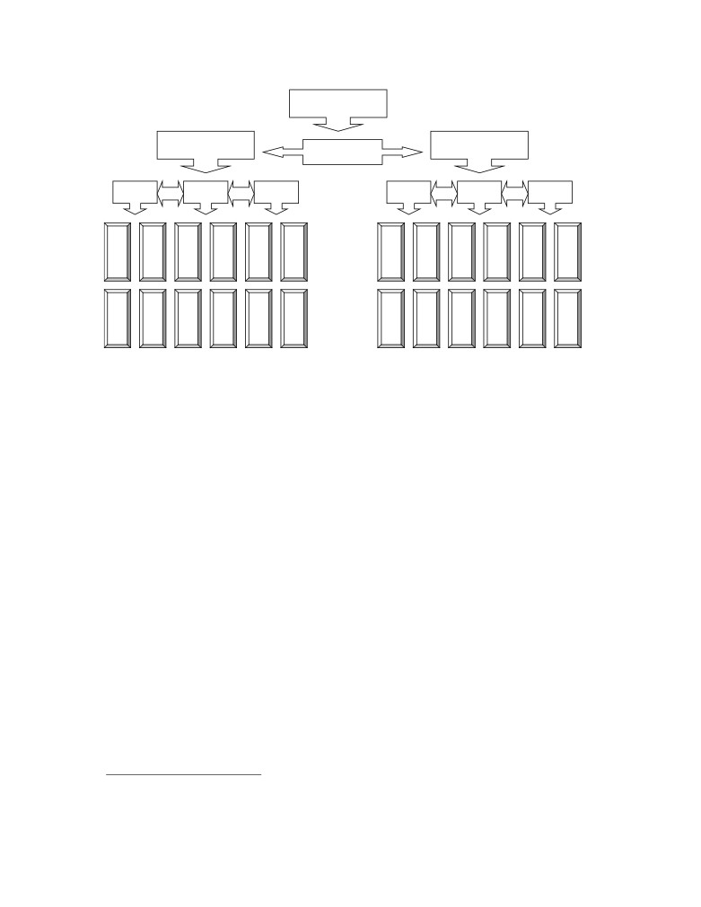
══════════════THEORY AND THE SMART MODEL═══════════════

A-list year X

Large

Small

Divide

B/P H

B/P M

B/P L

B/P H

B/P M

B/P L

Figure 3.4 SMART method for sorting portfolios.

3.10.2 Other similar research

We could not find many other articles studying the combinations of anomalies that we have

used to create portfolios. One article that describes a similar approach was Market Efficiency

in an Irrational World by Daniel & Titman in 1999. Their study was based on CRSP and

COMPUSTAT data on the American market. They concluded that investor overconfidence

generates momentum in stock returns, and the strongest effect would be found in stocks with

much ambiguous information that are hard to interpret. Momentum effects were stronger for

growth stocks than for stable stocks. They found that strong abnormal returns were possible

and could not be attributed to risk. They tested a weak form of market efficiency called

adaptive efficiency. It allows for profit opportunities in historical data, but requires these

profits to evaporate when they become apparent. However their tests rejected the possibility

of US equity market being adaptive efficient. The effect of selecting stocks by Size, B/P and

Momentum was a strong abnormal return, even during the 1990s when the individual effects

of these three factors were well known and did not disappear.⁶¹ We have not fund any report

like this one done for the Swedish market, which motivates the empirical part of this thesis.

There are however a few studies that are related to size and B/P;

Gunnarsson and Åkesson studied ”Firm Size Effect and PE Effect on the Stockholm Stock

Exchange” between 1994-1999. The size effect was the only significant factor and produced

abnormally high risk-adjusted returns.⁶²

Bacchus, Broström, and Leveau found a small firm effect between 1982-1996 which had a

yearly average of +6,51% to +7,89% with 5% significance. The efficient market hypothesis in

the semi-strong form is rejected for the Stockholm stock exchange since they could confirm

⁶¹ Daniel, K. Titman, S. Market Efficiency in an Irrational World (Financial Analysts Journal, vol. 55 No 6

November/December 1999), pp. 28-40

⁶² Gunnarson, P & Åkesson, C (2000). Firm Size Effect and PE Effect on the Stockholm Stock Exchange. Master

Thesis (abstract). Department of Business Administration, Lund University. (2006-04-17)

══════════════THEORY AND THE SMART MODEL═══════════════

abnormal returns with publicly available information. However they rejected the hypothesis

that institutional ownership had any connection with the small firm effect.⁶³

Claesson, Kantmark, Nyman and Sjöslätt concluded that the B/P ratio is to some degree

related to abnormal returns, and the correlation is especially strong during the month of

January. However they did only find the relationship in a small sample of the studied stocks.

They could not confirm that B/P would be a viable tool for selecting stocks with abnormal

returns on the Swedish stock market. Due to restrictions in their research they encourage more

research regarding the B/P ratio and its connection to returns on the Swedish market before

any definite confirmation of correlation can be determined. Furthermore they could not

confirm that Size had any effect on returns.⁶⁴ Their results were therefore quite different from

the majority of findings in the American research articles as well as the two Swedish studies

mentioned above. It should be said that the third of this is the most advanced regarding both

data treatment and statistics.

3.11 Risk measures for SMART

When measuring the performance of portfolios many claim that absolute returns is not a very

good measure. But it’s still what you get in return that shows up on your bank account

regardless of the risks taken to get those returns. However it’s often more interesting to know

if the high returns were actually a product of skill from the portfolio manager or if it was just

a result of taking on more risk. We will also present a ranking of the best SMART

combinations based on returns compared to risks taken, therefore we need to introduce the

reader to the topic of risk measures, and specifically the Sharpe ratio which we will use.

In investment you often want to see how high risks were taken to achieve a special return. For

this reason several risk measures have been developed such as the Sharpe ratio, CAPM Alpha

and Beta, Treynor ratio, Information ratio, and Style-adjusted alpha. There are no ideal risk

measures, they all have drawbacks.⁶⁵ In our thesis we will only use the Sharpe ratio for

several important reasons we will discuss in a moment. But first we must describe the

standard deviation.

3.11.1 Standard deviation

The Standard Deviation σ is a measure of the volatility of portfolio returns. More specifically

it’s a measure of the average difference between values of the data in a set. If the values

(returns) are at a similar level the σ will be low. It will indicate how much the returns goes up

and down during a specified time period. Therefore it can be used to quantify the risk for

investments.⁶⁶

⁶³ Bacchus, B. Boström, J. Leveau, D. (1998). Småbolagseffekten på Stockholms Fondbörs (Small firm effect on

the Stockholm stock exchange). Bachelor Thesis (abstract). Department of Business Administration, Lund

University. URL: http://www.fek.lu.se/ERB.asp?EB_iid={CBFFB5F5-EF15-462A-9358-8AD845DBD559}

&EB_rid=3&action=detailed&id=8082 (2006-04-17)

⁶⁴ Claesson, J. Kantmark, R. Nyman, J. Sjöslätt, Ö. (2004). Book-to-Market: Avkastar eller förkastar? (Book-to-

Market: Returns or Rejection?), Department of Business Administration, Lund University.

URL: http://www.fek.lu.se/ERB.asp?EB_iid={CBFFB5F5-EF15-462A-9358-8AD845DBD559}

&EB_rid=3&action=detailed&id=11752 (2006-04-17)

⁶⁵ Siegel, L. B. Kroner, K. F. Clifford, S. W. In Pursuit of Performance: The Greatest Return Stories Ever Told.

(Barclays Global Investors - Investment Insights, Vol. 4 No 1 August 2001), pp. 4-9

⁶⁶ Anderson D. R. Sweeney D. J. Williams T. A. Statistics for Business and Economics. (Ohio: Thomson

Learning), p. 86-87

══════════════THEORY AND THE SMART MODEL═══════════════

3.11.2 Sharpe ratio

The simplest way to obtain risk-adjusted returns is to divide the excess returns (over the risk

free rate) by the standard deviation, and this is exactly what the Sharpe ratio is. It simple but

yet very powerful. This ratio was developed by the Nobel Prize winner William F. Sharpe and

below you see the definition⁶⁷:

Sp = (r_p-r_f)/ σ_p

Sp = Sharpe ratio of portfolio p.

r_p= Mean return on portfolio p.

r_f

= Mean return on the risk free asset, in our thesis defined as short-term treasury bills. We

have used the mean of Riksbanken’s yearly values 1995-2005 which gave us an average risk

free rate of 4,06%.

σ_p = Standard deviation of returns on portfolio p.

The Sharpe ratio is used to value how well the return of a portfolio compensates the investor

regarding risks taken to achieve this. If we have two portfolios with the same return, the

portfolio with the highest Sharpe ratio gives more return for the same risk. It’s therefore

usually recommended to select the portfolio with the highest Sharpe ratio.

3.11.3 Reasons for selecting the Sharpe ratio

The Sharpe ratio has the benefit that very different investment strategies can be analysed with

it. It is especially useful for measuring risk for unusual investment strategies for which Beta

or CAPM is not useful. As we pointed out earlier in this thesis we are building our strategy on

anomalies which CAPM have problems to explain. CAPM Alpha and Beta measuers the risk-

adjusted returns only if the CAPM is valid, or in other words if it is an accurate model for

expected return. We believe it is generally an acceptable tool even if it’s not perfect. But for

our thesis with this special investment strategy, that builds portfolios according to SMART, it

is probably not very usefull for us. Treynor ratio also uses Beta and won’t be of much aid

either. The Sharpe ratio avoids this problem by using standard deviation instead of Beta.

According to Barlcay’s Investment Insights it’s the closest thing to a universal risk measure

that does not depend on the strategy used when analysing the results⁶⁸. Our conclusion is

therefore that the Sharpe ratio is the most appropriate for this study.

⁶⁷ Siegel, L. B. Kroner, K. F. Clifford, S. W. In Pursuit of Performance: The Greatest Return Stories Ever Told.

(Barclays Global Investors - Investment Insights, Vol. 4 No 1 August 2001), p. 4

⁶⁸ Siegel, L. B. Kroner, K. F. Clifford, S. W. In Pursuit of Performance: The Greatest Return Stories Ever Told.

(Barclays Global Investors - Investment Insights, Vol. 4 No 1 August 2001), p. 5

══════════════THEORY AND THE SMART MODEL═══════════════

3.11.4 Example of the Sharpe ratio

The Sharpe ratio is benchmark independent, which means we don’t actually need to compare

the results to the index. As a practical reference for the Sharpe ratio we present a Top 20 table

of the best risk-adjusted fund performances on the US market between 1980-2000.

Table 3.2 Example of Sharpe ratio ⁶⁹

3.12 Hypotheses

When testing a hypothesis you need two versions, one null hypothesis H-0 and one alternative

hypothesis H-1. In practise we present two competing statements and test which one is

correct. The H-1 will only be accepted if the H-0 is rejected.⁷⁰ A pure statistician would never

admit that he “accepts” a hypothesis, he only rejects null hypotheses. If he can reject H-0 he

would not agree that he could accept H-1, but would much rather conclude that it is possible

that H-1 is true but we can’t be completely sure. However this is not a very practical approach

if we actually want to say something about reality, and not only confirm that something is not

following a special rule. Furthermore it’s common to see language in non-statistical reports

that describes H-1 as accepted because it’s more easy for people to understand the results

then. If something is true in almost all cases most people would agree that there is a strong

support for the alternative hypothesis even if exceptions may exist which violates it. In reality

things are very rarely black or white but usually also have grey zones. The somewhat ironic

conclusion we can make, from this paragraph of text, is that we for sure can reject the

hypothesis that a statistician constructed the universe we live in. This text is probably

approaching a grey zone for how hilarious a scientific study may be allowed to be.

⁶⁹ Siegel, L. B. Kroner, K. F. Clifford, S. W. In Pursuit of Performance: The Greatest Return Stories Ever Told.

(Barclays Global Investors - Investment Insights, Vol. 4 No 1 August 2001), p. 5

⁷⁰ Watsham, T. J. & Parramore, K. Quantitative Methods in Finance. (Oxford: Thomson Learning), p. 170

══════════════THEORY AND THE SMART MODEL═══════════════

Anyway we now have the theoretical foundation for establishing the null hypothesis and the

alternative hypothesis for the testing of the SMART model:

• Hypothesis (H1-0): SMART will not discover one or more combinations that can

produce abnormal average returns.

(null hypothesis)

• Hypothesis (H1-1): It is possible to earn abnormal average returns by using one or

more of the combinations suggested by SMART.

(alternative hypothesis)

By abnormal returns we mean returns higher than AFGX General Index during the

period. AFGX is Sweden’s oldest stock index. It measures the average return and is a

good benchmark to compare Swedish stock portfolios against. It’s a wighted index and

each stock’s value is in proportion to its market value. From 1998 it also includes the O-

list, not only the A-list.⁷¹

We also formulate these additional hypotheses:

• Hypothesis (H2-0): Returns are not related to Market Value (Size).

• Hypothesis (H2-1): Returns are related to Market Value (Size).

• Hypothesis (H3-0): Returns are not related to the B/P ratio.

• Hypothesis (H3-1): Returns are related to the B/P ratio.

• Hypothesis (H4-0): Returns are not related to Momentum.

• Hypothesis (H4-1): Returns are related to Momentum.

⁷¹ AFGX, http://bors.affarsvarlden.se/afgx/aboutafgx.aspx?settings=afv , (2006-05-08)

════════════DATA MANAGEMENT AND TREATMENT═════════════

4 DATA MANAGEMENT AND TREATMENT

This chapter will describe how we collected the data, which problems emerged and

how we dealt with it and also what implications our choices have for the results

The SIX-Trust database. SIX-Trust is foremost an information - and analysis tool for people

active in management, analysis and trading in the Nordic capital markets. Apart from current

financial information, the database also contains historic data from 1979. With the arithmetic

function built into the database, commands can be used to adjust the information to the user,

for example by dividing or multiplying variables. The information contained in the database is

collected from yearly- and quarterly reports and is processed by the staff of SIX.

We have used SIX Trust 1.1-6 to collect the stock specific data for this thesis. The data

collected for each stock on the OMX A-list is: Market Value (MV) - used as a proxy for the

company Size, Price - used for calculating returns and the ratio Price-to-Book (P/B),

transformed by taking 1/(P/B) to get the inverse Book-to-Market (B/P) - used for screening

out stocks since it’s been documented that this ratio alone has a significant effect on returns

when used as an investment strategy. Additionally we have gathered Momentum data - used

for ranking stocks on their trend over the last 12 months. We will use all of these to rank and

create portfolios. The period studied is 1995-2005 but the data collected ranges from the years

1994-2005 (since portfolio creation is based on the development during the year prior to the

formation of portfolios). Sometimes data is not available for all stocks because they have not

existed during the whole period and sometimes data for each of the factors mentioned above

are not available.

Two databases containing accounting variables are available for students at Umeå University:

Six Trust and Thompson DataStream. We worked mostly with the former because it was

possible to run the database from a laptop over the school’s wireless network. DataStream on

the other hand was only accessible from the university library’s computers which were

unacceptably slow to work with. We also found that Six Trust was the more comprehensive of

the two and as we wanted consistency in our data gathering, we used DataStream almost

exclusively to double check numbers obtained from the Six Trust database that seemed

questionable. As the database is completely command based, you have to know the right

commands and the ticker names for the companies in it to be able to work with it. This meant

that it took us some time to figure out how to get a hold of the necessary data, but after

extensive usage of the online help and some phone support we were finally able to master the

database.

To obtain a proper measure of Book-to-Market values for the companies in our sample we

used the built in function KURS/JEK which divides the value of a company by the adjusted

equity, defined as reported equity minus proposed dividend + 72 % of untaxed reserves. The

exact command used was: TAB ÅR KURS/JEK ticker F 1994. To get the market values we

used the command BV Ticker which multiplies the share price by the number of outstanding

shares. The exact command was: TAB BV ticker F 1994 Finally, the price momentum was

given by the formula TAB ÅR / - Ticker LAG 1 Ticker LAG 1 Ticker F 1994, where lag 1

means that you get the number one time period ago, in this case one year.

════════════DATA MANAGEMENT AND TREATMENT═════════════

As mentioned, the database is command based, meaning that you type in commands to get the

desired output, there is a theoretical risk of typing the wrong commands. In reality however,

this risk can be argued to be very small. First of all, for practical matters the commands do not

resemble each other, meaning that the risk of by chance typing in a different command than

the intended one is virtually non existent. The other possible scenario would be writing the

wrong command, for example the command for size when we were actually looking for the

Book-to-Market value. Fortunately, because the values of our investigated variables are very

far from each other, this risk can be dismissed. As we see it, the only case where there was a

realistic chance of any mistakes being made, would be in the formula used to calculate

momentum. As we did not have to type the command every time but merely press the up-

arrow to get the last written command, there was no risk of making any mistake with the

formula. The potential error would be to use the wrong ticker somewhere in the formula, for

example: TAB ÅR / - assa-b LAG 1 assa-b LAG 1 asg-b. As this risk was very obvious, we

were careful not to make this mistake and we would not be lying saying that we are at least 99

percent certain that this did not happened. And even if it would have, it should distort our set

of data in a way that resulted in systematically false results as the errors would have been

random.

4.1 Data management

The data from Six Trust could easily be copied and pasted into Excel - which we later used to

sort securities into portfolios - so there was no risk of mistyping when transferring the data.

Neither was there any risk of mixing up the company names as the ticker name of the

company was copied together with the data. There was however a risk related to the pasting of

data. Because we did not get figures over momentum, size and Book-to-Market over every

year, there was the possibility of pasting numbers into the wrong row, or effectively including

the data in the wrong year. This risk would probably be very large if it was not for the fact

that there was a sort of double checking taking place as one of us was responsible for finding

data over size and the other of finding data over momentum and Book-to-Market. As we

finally pasted all of our data into the same Excel sheet, with all data related to a given

company in the same column, it was easy to spot cases where data over one variable was

given for different years than the other variables. In fact, several errors were detected but were

very easily corrected. For any data to be pasted in the wrong year it would take that the same

exact mistake would be made on three times, by two different persons.

The likelihood of this happening will of course finally have to be decided upon by the reader,

but we the authors, would deem the likelihood of the series of events, necessary for any

mistakes in this area to have been made, to be very slim. It should also be pointed out that

even if a few mistakes were in fact made, it should not significantly affect the final results, it

would rather act as a small noise that would have only a slightly negative effect on the

accuracy of our results.

4.2 Potential problems regarding portfolio creation

In the empirical part of this thesis we will create portfolios each year during the period based

on the sample of stocks with available information for each of the factors Size, Price and P/B.

The exact portfolio construction procedure will be described in more detail later. For now it’s

enough to know that we will use a model called SMART to guide us in this task. If a stock

has a gap in any of these factors for a year the stock will be excluded from any possible

portfolio combination that year. If the stock existed for that specific year but our source

doesn’t have sufficient data there is not much we can do about it, the best thing to do then is

════════════DATA MANAGEMENT AND TREATMENT═════════════

to treat the stock as if it didn’t exist. This may in theory lead to a slight bias in our results but

this will be discussed later in more detail.

There are a several other known problems that researchers need to be aware of when creating

portfolios. Depending on how the study is done you will usually be subject to one or several

of them, it’s very hard to avoid all the potential problems and biases. As we can not fully

avoid them, it is important to make the reader aware of the most relevant ones that could

apply to our portfolio evaluation. Barber and Lyon identified the following important biases:

New listing bias, Measurement Bias, Rebalancing bias, Skewness bias, and Survivorship

bias.⁷²

Measurement bias. Depending on the using of cumulative returns or buy and hold returns the

calculation of long-run returns will become skewed in different ways. When using cumulative

returns, the returns from all the years in the sampling period are simply added together. Buy

and hold returns are calculated by multiplying the returns of each year. The difference

between the two methods is that the former ignores compounding while the latter includes the

effect of this. The fact that compounding is ignored when using cumulative returns skews the

results of tests long-run returns in favour of volatile portfolios or individual shares. The way it

does so can be shown with a trivial example: If the return on a portfolio in year one is 20 %

and in year two - 5 %, then the cumulative return will be 0.2 + (-0.05) = 15 %, while the buy

and hold returns will be ((1+0.2) x (1-0.05)) - 1 = 14 %. When holding portfolios over several

time periods, the cumulative return will be higher than the buy and hold return if the returns

are volatile enough and lower if the volatility is low enough. If we repeat the example above

with 15 % return for the first year and 10 % in the second year the cumulative return will be

25 % while the buy and hold return will be 26.5 %, this time higher than the cumulative

return. This is what is called measurement bias in cumulative returns. Because of the

skewness just described, cumulative returns are a biased predictor of long run portfolio

performance. When volatility is low enough, it underestimates long run returns and when it is

low enough, long run returns are overestimated. This becomes a problem when measuring the

return on a portfolio against a market index because the portfolio is very likely to experience

higher volatility than the index. This way, the long-run performance of the portfolio will be

overestimated.⁷³ We have mainly used cumulative returns to evaluate portfolios but we have

also graphed the buy and hold performance of the of the most interesting portfolios in the

analysis of the results. In appendix, graphs over buy and hold returns for all portfolios can be

found.

Rebalancing bias. To avoid the measurement bias inherent in the use of cumulative returns,

buy and hold returns can be used instead. There is however problems associated with this way

of calculating returns as well. One special problem with using buy and hold returns arises

when measuring the return of a portfolio against an equally weighted market index. Because

an equally weighted index needs to be rebalanced after each time period, for example each

day, or month, it means that it will have to remove holdings of the stocks that have beaten the

index and increase holdings stocks that have underperformed to index. When using short

observation periods such as days or months, there is a risk of bid ask bounce in the calculation

of index returns. This gives rise to a rebalancing bias. This bias comes about because it is

more likely that the shares with high returns in period t-1 are more likely to have a closing

transaction at the posted ask price, but are equally likely to have a closing transaction at the

⁷² Barber, B.M. & Lyon, J.D. Detecting Long-run Abnormal Stock Returns: The Empirical Power and

Specification of Test Statistics (Journal of Financial Economics, Vol. 43 no 3 1997), pp. 341-372

⁷³ Op. Cit

════════════DATA MANAGEMENT AND TREATMENT═════════════

bid and the ask price in period t. This causes a reversal effect to come about which leads to a

positive bias in the return on the index. This happens because portions of the good performers

in period t-1, who are more likely to perform badly in period t, are sold off while portions of

the bad performers in period t-1, that are more likely to perform well in period t, are bought.

As mentioned, this effect works more strongly the shorter the evaluation periods being used.

It is also stronger for infrequently traded stocks. Using a market weighted index as reference

such as AFGX, which is what we have chosen to do, eliminates the problem of rebalancing

bias. The problem could however arise when we use the total sample of stocks as a reference

against our portfolios, but as we are looking at yearly returns, it is very unlikely that this

potential bias would make an effect.⁷⁴

Skewness bias. A problem affecting statistical tests on both cumulative and buy and hold

return is skewness bias. This problem arises because abnormal returns or departures from the

sample return, are generally not normally distributed but have a positive skewness, meaning

that that a the sample median is lower than the sample mean, which means that a few extreme

returns bump up the mean. A sample with a mean return higher than average (in our case a

portfolio performing better than index) will because of this have a greater chance of

containing one or more of these extreme positive observations. As a result, statistical tests will

overestimate the true standard deviation of samples with returns higher than average. In short,

there is a positive relationship between sample returns and standard deviation: The higher the

return the higher the standard deviation will be on average. This may affect our results in the

way that the estimated Sharpe ratios, which we will discuss in chapter 3.11, will be lower than

the true Sharpe ratios for the best performing portfolios and higher for the worst performing

portfolios.⁷⁵

New listing bias. A fourth bias arising when using a reference index is new listing bias. This

bias comes about when newly listed shares either under- or overperform the index. The reason

why this happens is because newly listed firms will be part reference index before they are

included in the sample, which usually happens in the beginning of a month, or as in our case

year. Newly listed firms have been shown to underperform index which means that the returns

on our sample portfolios may be positively biased. However, as the main purpose of our thesis

is to evaluate portfolios against each other and not against the market index, it does not affect

our evaluation in any central way.⁷⁶

Survivorship bias (generates positive bias). Since we rearrange portfolios each year, we might

introduce a problem that could affect the outcome of this thesis to some extent. It’s called

Survivorship bias and emerge when poorly performing companies go bankrupt or for some

other reason are deleted from the stock market list. Only a successful and well managed firm

will stay on the list year after year (in our case the A-list). Sometimes companies become

transferred to the “Observation list” if there is a problem or there needs to be an investigation

to see if the company holds up to the rules and regulations of the stock exchange. Therefore

we must be aware that there could be a positive bias in our result since only surviving firms

are candidates for future portfolio selections, the bad companies will not stay on the list and

we will be unable to select them. Barber & Lyon report that this bias is actually proposed as

an explanation of the B/P effect and refers to Kothari, Shanken and Sloan from 1995, but

Barber & Lyon also state that this is disputed by Chan, Jegadeesh and Lakonishok in their

⁷⁴ Barber, B.M. & Lyon, J.D. Detecting Long-run Abnormal Stock Returns: The Empirical Power and

Specification of Test Statistics (Journal of Financial Economics, Vol. 43 no 3 1997), pp. 341-372

⁷⁵ Op. Cit

⁷⁶ Op. Cit

════════════DATA MANAGEMENT AND TREATMENT═════════════

article from the same year, which found the survivorship bias in COMPSTAT data to be

small.⁷⁷ Because of the concern that survivorship bias would be the reason for the observed

premium on high book-to-market shares we decided to make small test to see it there were

any support for the survivorship bias hypothesis in our material. The test is described in detail

in chapter 8.4 and in short we can conclude that there is no evidence pointing towards any

survivorship bias in our data. The book-to-market effect appears to work in the same direction

in the last year of listing as in the rest of the data, with a premium for firms with high ratios.

Continuously compounded- or simple returns. In our evaluation of portfolio performance we

have chosen to work with simple yearly returns as opposed to monthly, daily or continuously

compounded returns. The primary reason behind this choice is that we are evaluating a

strategy with one year holding periods. There is also a practical reason for using simple yearly

returns. Compounding returns with shorter intervals would bring a negative bias on the

returns on our portfolios. Unless all securities or portfolios have equal return for each period

of compounding (that is assumed to be shorter than the evaluation period) the mean return for

all shares or portfolios will be lower than the index return.⁷⁸

⁷⁷ Barber, B.M. & Lyon, J.D. Detecting Long-run Abnormal Stock Returns: The Empirical Power and

Specification of Test Statistics (Journal of Financial Economics, Vol. 43 no 3 1997), p. 356

⁷⁸ Op. Cit

═════════EMPIRICAL EVALUATION OF THE SMART MODEL═════════

5 EMPIRICAL EVALUATION OF THE SMART MODEL

This chapter will present the empirical tests and evaluation of the SMART investment

model that will create the foundation for the analysis and conclusions

5.1 SMART 1995

Table 5:1 SMART 1995 (average: 5,17)

SIZE

B/P(H)

B/P(M)

B/P(L)

MOMENTUM

6,53

-4,06

6,57

-9,78

3,45

15,83

5,73

1,43

16,77

-0,06

1,37

18,24

Table 5:3 SMART 1995 mean of main factors

Table 5:2 SMART 1995 Ranking of portfolios

Large:

3,09

Small:

7,25

S-L-L

S-L-H

L-L-L

L-L-H

L-H-H

S-H-H

18,24

16,77

15,83

6,57

6,53

5,73

B/P H

0,60

B/P M

0,55

L-M-L

S-M-H

S-M-L

S-H-L

L-M-H

L-H-L

B/P L

14,35

3,45

1,43

1,37

-0,06

-4,06

-9,78

MOM H

5,50

5.2 SMART 1996

MOM L

4,84

Table 5:4 SMART 1996 (average: 40,29)

SIZE

B/P(H)

B/P(M)

B/P(L)

MOMENTUM

54,35

44,35

42,57

50,04

25,13

36,14

20,99

39,62

30,15

46,68

31,75

61,70

Table 5:6 SMART 1996 mean of main factors

Table 5:5 SMART 1996 Ranking of portfolios

Large:

42,10

Small:

38,48

S-L-L

L-H-H

L-H-L

S-H-L

L-M-H

L-L-H

61,70

54,35

50,04

46,68

44,35

42,57

B/P H

43,02

B/P M

35,21

S-M-H

L-L-L

S-M-L

S-L-H

L-M-L

S-H-H

B/P L

42,64

39,62

36,14

31,75

30,15

25,13

20,99

MOM H

38,67

MOM L

41,91

═════════EMPIRICAL EVALUATION OF THE SMART MODEL═════════

5.3 SMART 1997

Table 5:7 SMART 1997 (average: 16,09)

SIZE

B/P(H)

B/P(M)

B/P(L)

MOMENTUM

27,25

23,90

34,75

22,22

5,60

-1,95

9,44

5,73

26,69

4,61

23,30

11,57

Table 5:9 SMART 1997 mean of main factors

Table 5:8 SMART 1997 Ranking of portfolios

Large:

18,63

Small:

13,56

L-L-H

L-H-H

S-L-H

L-M-H

S-M-L

L-H-L

34,75

27,25

26,69

23,90

23,30

22,22

B/P H

15,88

B/P M

14,63

S-L-L

S-H-H

S-M-H

L-M-L

S-H-L

L-L-L

B/P L

17,77

11,57

9,44

5,73

5,60

4,61

-1,95

MOM H

21,29

MOM L

10,89

5.4 SMART 1998

Table 5:10 SMART 1998 (average: -10,56)

SIZE

B/P(H)

B/P(M)

B/P(L)

MOMENTUM

-16,11

-10,80

25,93

-26,52

-2,01

-7,17

-10,91

-23,21

-12,30

-26,89

-12,44

-4,23

Table 5:12 SMART 1998 mean of main factors

Table 5:11 SMART 1998 Ranking of portfolios

Large:

-6,11

Small:

-15,00

L-L-H

L-M-L

S-L-L

L-L-L

L-M-H

S-H-H

25,93

-2,01

-4,23

-7,17

-10,80

-10,91

B/P H

-20,10

B/P M

-12,11

S-L-H

S-M-L

L-H-H

S-M-H

L-H-L

S-H-L

B/P L

0,56

-12,30

-12,44

-16,11

-23,21

-26,52

-26,89

MOM H

-7,90

MOM L

-13,21

═════════EMPIRICAL EVALUATION OF THE SMART MODEL═════════

5.5 SMART 1999

Table 5:13 SMART 1999 (average: 36,88)

SIZE

B/P(H)

B/P(M)

B/P(L)

MOMENTUM

35,38

38,71

58,78

64,64

28,17

33,45

56,51

27,73

7,02

31,31

29,73

31,14

Table 5:14 SMART 1999 Ranking of portfolios

Table 5:15 SMART 1999 mean of main factors

Large:

43,19

L-H-L

L-L-H

S-H-H

L-M-H

L-H-H

L-L-L

Small:

30,57

64,64

58,78

56,51

38,71

35,38

33,45

B/P H

46,96

S-H-L

S-L-L

S-M-L

L-M-L

S-M-H

S-L-H

B/P M

31,09

31,31

31,14

29,73

28,17

27,73

7,02

B/P L

32,60

MOM H

37,36

MOM L

36,41

5.6 SMART 2000

Table 5:16 SMART 2000 (average: -3,89)

SIZE

B/P(H)

B/P(M)

B/P(L)

MOMENTUM

-22,65

-8,38

-0,78

-3,56

5,43

-19,74

0,31

1,77

2,17

-12,55

-6,05

17,30

Table 5:18 SMART 2000 mean of main factors

Table 5:17 SMART 2000 Ranking of portfolios

Large:

-8,28

Small:

0,49

S-L-L

L-M-L

S-L-H

S-M-H

S-H-H

L-L-H

17,30

5,43

2,17

1,77

0,31

-0,78

B/P H

-9,61

B/P M

-1,81

L-H-L

S-M-L

L-M-H

S-H-L

L-L-L

L-H-H

B/P L

-0,26

-3,56

-6,05

-8,38

-12,55

-19,74

-22,65

MOM H

-4,59

MOM L

-3,19

═════════EMPIRICAL EVALUATION OF THE SMART MODEL═════════

5.7 SMART 2001

Table 5:19 SMART 2001 (average: 8,26)

SIZE

B/P(H)

B/P(M)

B/P(L)

MOMENTUM

22,91

-15,88

15,07

19,65

3,67

-17,52

54,05

14,87

12,51

5,62

-0,56

-15,30

Table 5:20 SMART 2001 Ranking of portfolios

Table 5:21 SMART 2001 mean of main factors

Large:

4,65

S-H-H

L-H-H

L-H-L

L-L-H

S-M-H

S-L-H

Small:

11,87

54,05

22,91

19,65

15,07

14,87

12,51

B/P H

25,56

S-H-L

L-M-L

S-M-L

S-L-L

L-M-H

L-L-L

B/P M

0,53

5,62

3,67

-0,56

-15,30

-15,88

-17,52

B/P L

-1,31

MOM H

17,26

5.8 SMART 2002

MOM L

-0,74

Table 5:22 SMART 2002 (average: -20,66)

SIZE

B/P(H)

B/P(M)

B/P(L)

MOMENTUM

-8,04

-16,60

-19,88

-27,69

-8,65

-62,40

-6,37

-8,65

4,51

-12,79

-21,66

-36,30

Table 5:24 SMART 2002 mean of main factors

Table 5:23 SMART 2002 Ranking of portfolios

Large:

-27,78

Small:

-13,54

S-L-H

S-H-H

L-H-H

S-M-H

S-H-L

L-M-H

4,51

-6,37

-8,04

-8,65

-12,79

-16,60

B/P H

-13,72

B/P M

-19,75

L-L-H

S-M-L

L-H-L

L-M-L

S-L-L

L-L-L

B/P L

-28,52

-19,88

-21,66

-27,69

-32,09

-36,30

-62,40

MOM H

-9,17

MOM L

-32,15

═════════EMPIRICAL EVALUATION OF THE SMART MODEL═════════

5.9 SMART 2003

Table 5:25 SMART 2003 (average: 30,94)

SIZE

B/P(H)

B/P(M)

B/P(L)

MOMENTUM

30,34

14,70

34,74

51,53

31,90

-5,97

32,82

20,10

20,91

97,23

16,01

27,08

Table 5:27 SMART 2003 mean of main factors

Table 5:26 SMART 2003 Ranking of portfolios

Large:

26,18

Small:

35,69

S-H-L

L-H-L

L-L-H

S-H-H

L-M-L

L-H-H

97,23

51,39

34,74

32,82

31,90

30,34

B/P H

52,94

B/P M

20,68

S-L-L

S-L-H

S-M-H

S-M-L

L-M-H

L-L-L

B/P L

19,19

27,08

20,91

20,10

16,01

14,70

-5,97

MOM H

25,60

5.10 SMART 2004

MOM L

36,27

Table 5:28 SMART 2004 (average: 19,80)

SIZE

B/P(H)

B/P(M)

B/P(L)

MOMENTUM

6,73

16,50

31,24

25,87

11,98

-3,88

13,64

27,90

-1,21

59,67

21,83

27,36

Table 5:30 SMART 2004 mean of main factors

Table 5:29 SMART 2004 Ranking of portfolios

Large:

14,74

Small:

24,86

S-H-L

L-L-H

S-M-H

S-L-L

L-H-L

S-M-L

59,67

31,24

27,90

27,36

25,87

21,83

B/P H

26,48

B/P M

19,55

L-M-H

S-H-H

L-M-L

L-H-H

S-L-H

L-L-L

B/P L

13,38

16,50

13,64

11,98

6,73

-1,21

-3,88

MOM H

15,80

MOM L

23,80

═════════EMPIRICAL EVALUATION OF THE SMART MODEL═════════

5.11 SMART 2005

Table 5:31 SMART 2005 (average: 39,69)

SIZE

B/P(H)

B/P(M)

B/P(L)

MOMENTUM

48,61

9,52

23,85

33,30

53,86

33,35

48,80

39,91

52,45

71,27

33,17

28,21

Table 5:33 SMART 2005 mean of main factors

Table 5:32 SMART 2005 Ranking of portfolios

Large:

33,75

Small:

45,64

S-H-L

L-M-L

S-L-H

S-H-H

L-H-H

S-M-H

71,27

53,86

52,45

48,80

48,61

39,91

B/P H

50,49

B/P M

34,11

L-L-L

L-H-L

S-M-L

S-L-L

L-L-H

L-M-H

B/P L

34,46

33,35

33,30

33,17

28,21

23,85

9,52

MOM H

37,19

MOM L

42,19

5.12 SMART mean results 1995-2005

Table 5:34 SMART 1995-2005 (average: 14,73, AFGX: 15,56)

SIZE

B/P(H)

B/P(M)

B/P(L)

MOMENTUM

16,85

8,36

22,99

18,14

12,28

0,01

20,46

13,38

14,52

24,01

10,59

15,16

Table 5:35 SMART 1995-2005 Summary for main factors

Winner

Average:

Factors:

(No. of Yrs)

T-test 95% confidence

interval t >1,673

Large:

13,11

Small:

16,35

0,62

2,22

2,84

0,81

0,82

4,56

B/P H

19,86

1,77

0,5

0,01

B/P M

11,15

1,74

1,61

0,12

B/P L

13,17

This gives information

about how probable it is

MOM H

16,09

that the returns are not

MOM L

13,37

only random deviations.

═════════EMPIRICAL EVALUATION OF THE SMART MODEL═════════

The theoretically best combination (S-H-H) situates itself at an honouring 3:e place. The most

pronounced effect when locking at raw returns is not unexpectedly high B/P. Not that

surprising we se L-L-L at the very bottom, producing almost no return at all. The size effect

seem to be quite a bit lower on the Swedish market compared to American articles, the same

goes for momentum, which may be due to the 12*12 momentum we have used which is not

the optimal but required in this study for practical reasons.

5.13 SMART Sharpe ratio 1995-2005

For reference AFGX

index average for the

Table 5:36 Ranking by Standard Deviation

period was 15,56. Five

portfolios outperformed

S-H-L

L-H-L

L-L-L

S-L-L

L-H-H

S-H-H

the index: S-H-L, L-L-H,

S-H-H, L-H-L, L-H-H.

40,01

31,53

29,13

26,19

25,61

24,25

L-M-L

L-L-H

L-M-H

S-M-H

S-M-L

S-L-H

22,24

21,80

21,40

20,04

19,23

17,77

Table 5:37 Ranking by Sharpe Ratio

L-L-H

S-H-H

S-L-H

L-H-H

S-H-L

S-M-H

0,87

0,68

0,59

0,50

0,47

L-H-L

S-L-L

L-M-L

S-M-L

L-M-H

L-L-L

0,45

0,42

0,37

0,34

0,20

-0,14

Table 5:38 Ranking by Mean Returns

S-H-L

L-L-H

S-H-H

L-H-L

L-H-H

S-L-L

24,01

22,99

20,46

18,14

16,85

15,16

S-L-H

S-M-H

L-M-L

S-M-L

L-M-H

L-L-L

14,52

13,38

12,28

10,59

8,36

0,01

1000,00

800,00

AFGX

600,00

SMART

400,00

L-L-H

200,00

0,00

1995

1996

1997

1998

1999

2000

2001

2002

2003

2004

2005

Figure 5:1 Total return (buy and hold) from starting value of 100 for SMART (all portfolios), L-L-H and AFGX.

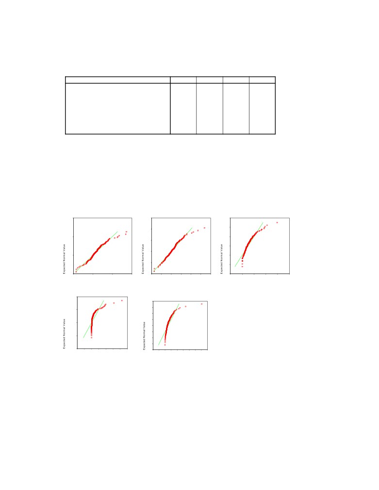
═════════EMPIRICAL EVALUATION OF THE SMART MODEL═════════

5.14 Correlation analysis for 1995-2005

Table 5:39 Summary of statistical data

Statistics

RET

MOM

Valid

678

Missing

Mean

15,3945

19219,57

,6370

,1376

Std. Deviation

41,01990

61172,95

,42260

,39719

Skewness

1,328

9,923

2,319

1,307

Std. Error of Skewness

,094

Kurtosis

4,405

129,807

14,843

4,308

Std. Error of Kurtosis

,187

As we know market value have very high positive skewness (because of a few huge

companies and many relatively small), this is not good for statistical tests requiring the data to

be normally distributed. The kurtosis is also very high (the curve is very high and has to much

weights to far out to the sides usually in clusters), but you can’t really discuss kurtosis when

the data has skewness. You need to have normal distribution to do that.

Normal plot for factors:

Normal Q-Q Plot of RET

Normal Q-Q Plot of MOM

Normal Q-Q Plot of BP

200

1,5

2,0

1,5

1,0

100

1,0

0,0

-,5

-100

-1,0

-100

100

200

-1,0

-,5

0,0

1,0

1,5

2,0

-1

Observed Value

Normal Q-Q Plot of MV

200000

Normal Q-Q Plot of P

500

400

100000

300

200

100

-100000

-100

-200

-200000

-300

-200000

200000

400000

-400

400

800

1200

-100000

100000

300000

500000

-200

200

600

1000

1400

Observed Value

Figure

5:2 Normal QQ plot for factors. Note: RET=Returns,

MOM=Momentum, BP=Book-to-Market,

MV=Market Value, P=Price at the beginning of each year.

We se that Returns and Momentum are closest to attaining the normal distribution criteria, but

none of the variables have a really good fit. If only a few observations on the tails are out of

line you can usually treat it as normally distributed and do standard statistic tests, but for

everyone except maybe momentum this is questionable and could lead to errors in the

analysis. There is however one trick we can do to get around the normal distribution problem

with the data. We can use Spearman rank-order correlation instead of the standard Pearson

═════════EMPIRICAL EVALUATION OF THE SMART MODEL═════════

correlation. They are quite similar but Spearman measures the linear association between two

variables that can be ranked (from lowest to highest) and can be used when the data does not

apply to normal distribution assumption⁷⁹. Therefore we can still use the actual values of the

variables.

5.14.1 Correlations calculation with actual-values 1995-2005

Table 5:40 Correlation with actual values

Correlations

RET

MOM

Spearman's rho

RET

Correlation Coefficient

1,000

-,014

,073*

-,047

Sig. (1-tailed)

,359

,028

,111

678

Correlation Coefficient

-,014

1,000

-,369**

,134**

Sig. (1-tailed)

,359

,000

678

Correlation Coefficient

,073*

-,369**

1,000

-,327**

Sig. (1-tailed)

,028

,000

678

MOM

Correlation Coefficient

-,047

,134**

-,327**

1,000

Sig. (1-tailed)

,111

,000

678

*. Correlation is significant at the .05 level (1-tailed).

Correlation is significant at the .01 level (1-tailed).

**.

We see that we have a significant correlation with Returns for B/P (at the 5% level). Market

Value is also strongly correlated with B/P and Momentum. We can not confirm that there is a

statistically significant correlation between Size-Returns or Momentum-Returns, they could

however still be dependent and follow a non-linear function. We initially also tried to do a

multiple regression analysis but it proved to be cumbersome task, both because of the

distribution problem and the fact the factors are correlated with each other and does not move

independently. Even after logarithmic transformation the factors did not have a good normal

fit. The results were difficult to decipher and we therefore limit ourselves to a correlation

table using Spearman to aid us in the analysis

However what we are most interested in for this thesis is how different combinations and

levels of the anomalies or factors can be used to create a profitable investment strategy, this is

what the SMART model is all about. And we will now move to the analysis to interpret the

results of that in more detail.

⁷⁹ Anderson D. R. Sweeney D. J. Williams T. A. Statistics for Business and Economics. (Ohio: Thomson

Learning), pp. 813-815

═══════════════════════ANALYSIS═══════════════════════

6 ANALYSIS

Presentation of the empirical findings and its connections to the theories

6.1 Analysis of the results

Lining up the winner portfolios for the individual years it can be seen that the results differ a

lot between the years. The portfolio characterised by small size, high book-to-market ratio and

strong momentum, the S-H-H which according to theory on the anomalies related to these

factor should be the best, is the winning portfolio only for one year. Over

Table 6:1 Winning

the eleven years, there are seven different winning portfolios. If we were

portfolios each

year

to look for some pattern, it would be that the winning portfolio of year t

in many cases resembles or is identical to the winner in year t-1. This is

1995 S-L-L

the case for 95-96, 97-98 2003-2005. Small stocks also outperform large

1996 S-L-L

in every year from 2000 to 2005. Another pattern is that in the bull

1997 L-L-H

market up until the IT-crash, most of the winning portfolios contain high

B/P shares while the pattern is the opposite in the next bull market. Other

1998 L-L-H

than that it is hard to find any general characteristics when looking at the

1999 L-H-L

results for the individual years.

2000 S-L-L

2001 S-H-H

When we look at the anomalies individually over the whole period, it can

2002 S-L-H

be seen that the results are much more in line with what we expected.

2003 S-H-L

What can be seen is that just as the small firm effect discussed in chapter

3.6 predicts, small firms dominate over large firms and the difference is

2004 S-H-L

quite significant; small cap stocks beat large cap stock by an annual

2005 S-H-L

average of more than 3 %. The momentum strategy discussed in chapter

3.7 also proves to be successful with high momentum stocks beating low

momentum stocks by a little less than 3 %. When we look at the results for the Book-to-

Market strategy, the results are not fully in line with what was expected; the portfolio with

high Book-to-Market ratios does indeed perform the best but it is followed the low book-to

market and not the medium as predicted as recalled from chapter 3.8. Still it is a decisive win

for the shares of the companies with high ratios over low ratios by more than 5.5 %.

Looking at the ranking of the twelve portfolios after their average return over eleven years we

find our predicted winner portfolio S-H-H at place number three, after the S-H-L and the L-L-

H portfolio. In figure

5:1 below the huge difference in performance between the two

portfolios can be seen. An interesting observation that can be made is that the two portfolios

yield about the same up until about the time of the burst of the IT bubble. From 2001 and until

the end of the evaluation on the other hand, the S-H-H portfolio makes an impressive climb

while the L-L-L portfolio decreases in value.

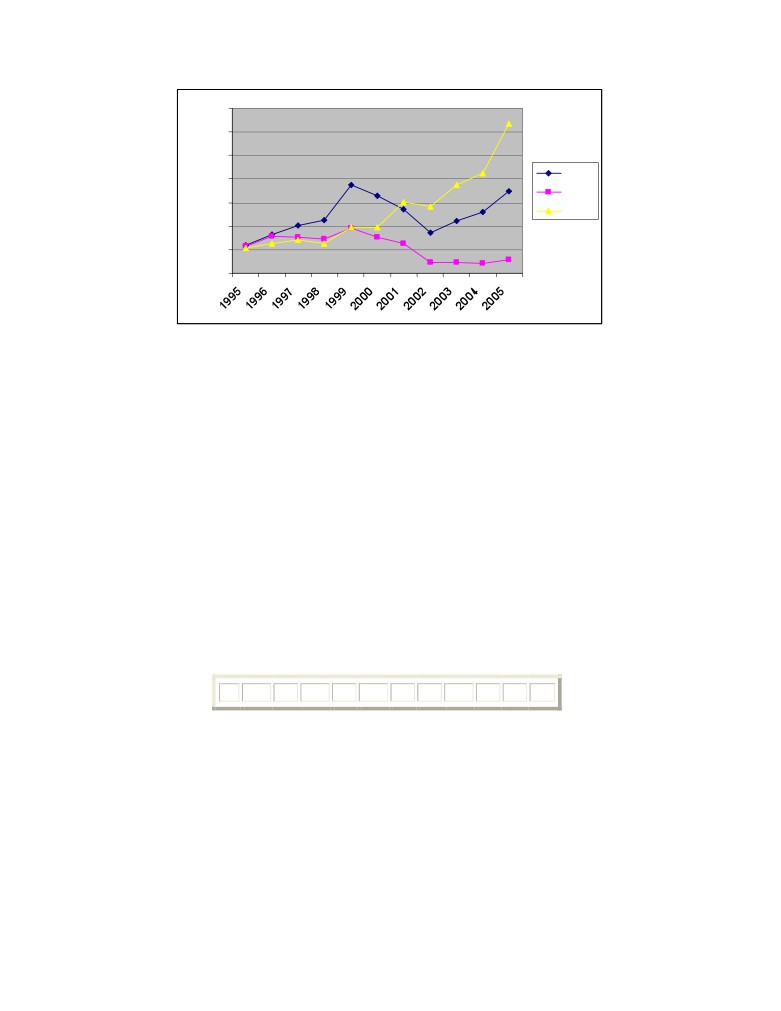
═══════════════════════ANALYSIS═══════════════════════

700,00

600,00

500,00

AFGX

400,00

L-L-L

300,00

S-H-H

200,00

100,00

0,00

Figure 6:1 Total return (buy and hold) from starting value of 100 S-H-H, L-L-L and AFGX.

The winning portfolio (S-H-L) has the two first characteristics expected to yield the highest

returns, namely small market cap and high Book-to-Market ratio, however it contained the

half of stocks in this category that had performed the worst over the year before formation.

The second best portfolio (L-L-H) goes against what theory suggests in two ways: it contains

large stocks with low Book-to-Market ratios. It does however contain stocks with high

momentum having performed the best over the year prior to portfolio formation. At the very

bottom we find the L-L-L portfolio, (or the triple loser portfolio as we prefer to call it). This

portfolio did not just perform the worst; it yielded a average of zero return over a ten year

period, 8 % less than the second worst performing portfolio.

The second worst performing portfolio was the L-M-H, having one characteristic suggested to

bring high returns, momentum, and one negative, size while the Book-to-Market ratio is

neutral. The third worst performer (S-M-L) also has one right, one wrong and one neutral:

small size, low momentum and neutral Book-to-Market ratio. Contrary to the portfolios

above, we can not reject that this underperformance is not due to chance. A good way to show

how the number of supposedly profit yielding characteristics possessed by the portfolios

impact on their rating is to give 1 point for correct, 0 for neutral and -1 for wrong. Doing so

takes the following form:

-1

-2

-1

-2

-3

Showing no particular pattern supporting our predictions except that the L-L-L portfolio is

placed last. The theory on these anomalies or effects does however not go into what the

expected result from combining them is so we really cannot say that the results speak against

theory. What we can say is that the above ranking does not bring any convincing evidence

against the efficient market hypothesis.

6.1.1 Bringing Sharpe into the picture

As risk is just as important as expected return when investing in stocks, in chapter 3.11 we

introduced the Sharpe measure which divides the difference between the return of a portfolio

and the risk-free rate by its standard deviation. Ranking portfolio performance after the

Sharpe measure we see that our predicted winner, the S-H-H portfolio steps up to second

═══════════════════════ANALYSIS═══════════════════════

place. The portfolio giving the best return, the S-H-L portfolio was subject to a very large

volatility over eleven years and is only the fifth ranking portfolio when ranking after the

Sharpe measure. The portfolio yielding the second best return, the L-L-H, steps up to first

place after adjusting for risk. According to theory, this portfolio should be one of the worst

performers but in our evaluation it gives a good return while not being overly volatile, only

slightly more than average. The fact that this portfolio performs so well is very interesting to

note. The portfolio giving the third best risk adjusted return is the S-L-H, which only produce

the seventh best return but with the lowest standard deviation of returns, only 17,8 %

compared to the average of about 25 %.

At the very bottom, once again we find the L-L-L portfolio. Only a negative standard

deviation could save this ill-performer from finishing last. The Sharpe measure gives a

somewhat strange measure for negative returns; it rewards high volatility as the standard

deviation is in the denominator. If we look at the standard deviation of the L-L-L portfolio,

we see that it is actually on of the portfolios experiencing the highest volatility; more than 29

% which makes it the third most volatile portfolio. The low return was predicted by theory but

not the high volatility, however, being only 4 % higher than the average and with the size of

our sample we really can not say that this is not due to chance. Second last from the bottom

we find the L-M-H portfolio. This one having the wrong size, neutral Book-to-Market and the

right momentum should according to theory be one of the medium performers so its

performance is worse than expected. Same goes for the portfolio giving the third worst Sharpe

measure the S-M-L: with one right, one neutral and one wrong its performance is also worse

than expected. Repeating the procedure of giving scores for the number of right and wrong

characteristics, this time placing the portfolios in order of Sharpe measure gives the following

form:

-1

-2

-3

This time the pattern looks a lot better than it did when we merely looked at the returns.

Except for the best performing portfolio scoring -1, the string of numbers looks a lot like how

it should according to theory. The best performing half of the portfolios score an aggregate of

7 while the worst performing half scores a total of -7.

In chapter 3.6 and 3.8 it was suggested that the size and the book-to-market effect would be

accompanied by an increase in risk. Even though the standard deviation is not a perfect

measure of risk it still captures much of the risk investors are subject to. In our evaluation,

small firms dominate large firms when ranking after Sharpe ratios and the same goes for high

book-to-market shares. In both cases the differences are substantial; the small firm shares in

our sample show a ratio of 0,79 while large firm shares only reach a ratio of 0,59. The high

book-to-market shares have a Sharp of 0,73 while the ones with low ratios only have 0,65.

This difference may not be enormous, but it definitely contradicts the suggestion that the

excess return on small firm stocks would simply be a compensation for increased risk.

6.1.2 Evaluation of interrelations

What the a regressions analysis would present does not show what SMART tells us about the

importance of combinations of the anomalies. We have clearly illustrated that it’s not only if

and how strong the correlation is between returns and the anomalies that are important, how

you combine the anomalies and the levels of them is also very important. Regressions can’t

illustrate that easily but the SMART model was developed to investigate this in more detail.

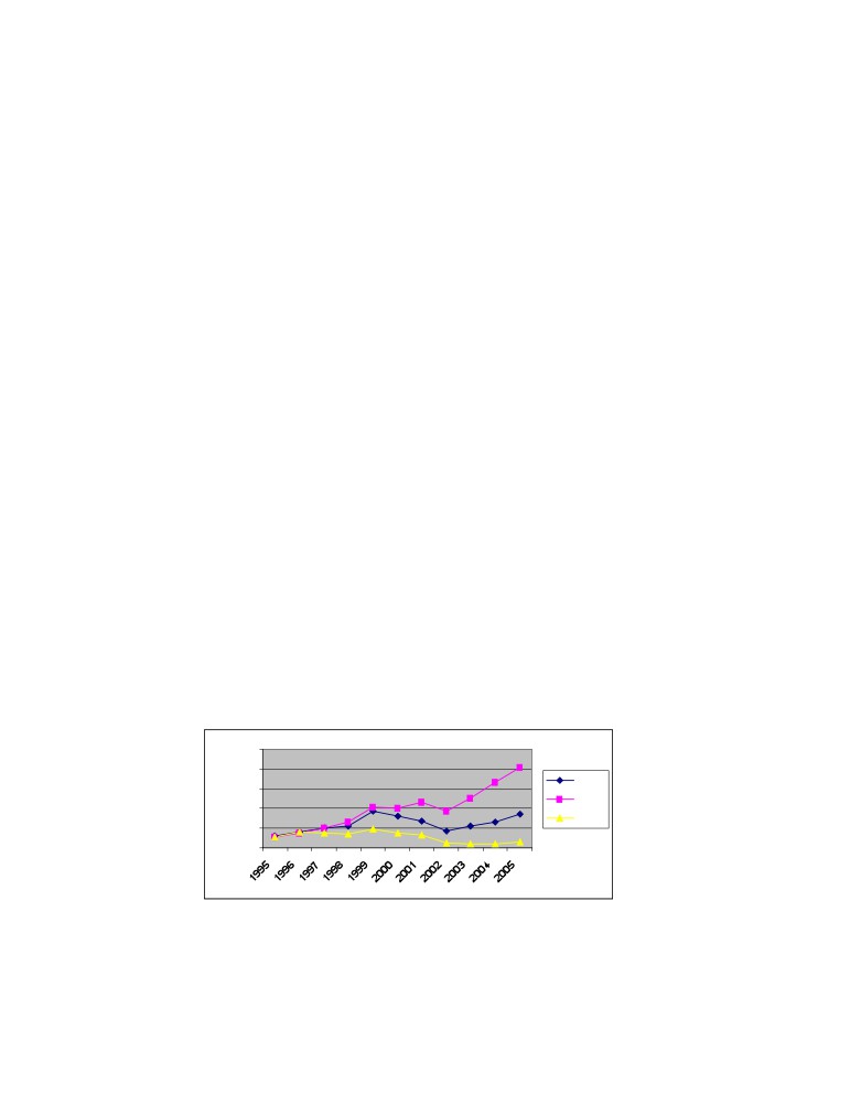
═══════════════════════ANALYSIS═══════════════════════

If we make an attempt to find any interrelations in the returns from the SMART model we see

that there appears to be no relation between the success of the Book-to-Market strategy and

size (even if the two individual factors are correlated in the statistical test shown in table

5.40). High-Book-to-Market shares on average gives about 1.5 times the return of the low

Book-to-Market share for both the group of large and small firms. When looking at the

relationship between momentum and Book-to-Market scores we find something interesting:

The momentum strategy appears to be much more effective for firms with low Book-to-

Market scores. For the group of shares with low book-to-market ratios, the difference in

return on high momentum shares and low momentum shares is over 11 % while actually

being negative by - 2,5 % for the group of shares with high Book-to-Market values. In figure

5:2 below, the performance of the L-L-L and the L-L-H portfolios are plotted. The return on

the two differs a lot from the very beginning of the evaluation period. It is interesting to note

that the portfolios share the characteristics of being large cap stocks with low book-to-market

ratios. The difference is that one of them contains the recent winners and the other the recent

losers. Applying a momentum strategy of selling short the losers and using the proceeds to

buy the winners on this subset of stock would have earned a huge profit. It appears as if the

momentum strategy works extra well for large cap stocks with low book-to-market ratios.

There appears to be a relationship between size and the success of a momentum strategy as

well: For large firms, the difference between the high and low momentum groups is 6 % while

there is only an insignificant difference of 0,5 % for the small firms.

Looking at how combining different anomalies affect the Sharpe-ratio we find that the

momentum effect is a lot stronger both for the large cap stocks as well as for the high Book-

to-Market stocks. For large firms the Sharpe ratio is more than twice as high for the high

momentum stocks as for the low momentum stocks. For small size firms the difference is only

a little less than a third in favour of the high momentum stocks. The Book-to-Market ratios

have an even stronger effect on momentum. For high Book-to-Market stocks the difference in

Sharpe measure between high and low momentum is quite small; only about a fourth better

for recent winners. For the low Book-to-Market shares on the other hand, there is a huge

difference: The Sharpe measure for the recent winners is about three and a half times that of

the recent losers. Of course, the large effect on the differences in Sharpe measures by size and

Book-to-Market are largely the effect of the terrible performance of the L-L-L portfolio.

1000,00

800,00

AFGX

600,00

L-L-H

400,00

L-L-L

200,00

0,00

Figure 6:2 Total return (buy and hold) from starting value of 100 for L-L-H, L-L-L, AFGX.

Averaging the total returns for small cap stocks, for high book-to-market stocks and for recent

winner stocks over the 11 year evaluation period arrives at a number of 17,4 %, Doing the

same for the stocks with the opposite characteristics gives an average of 13,2 %. This means

that the average difference in returns between stocks with the characteristics predicted to

═══════════════════════ANALYSIS═══════════════════════

provide the best returns and those with characteristics predicted to be least yielding is about

4,2 %. To evaluate the effectiveness of the SMART-Model compared to trading on the

anomalies separately one can contrast this difference with that between the S-H-H and the

L-L-L portfolio which is a striking 20,5 %. Combing the anomalies into the SMART-Model

gives a return 16 % greater than the average of simple trading strategies based on the three.

This shows that the SMART-Model has indeed found some interesting combinations of stock

characteristics that can be used for selection of stock and formation of portfolios.

6.1.3 Findings regarding B/P volatility

Since low B/P portfolios in our study have less standard deviation (or volatility) than high

B/P, contrary to the findings of Jensen, Johnson and Mercer⁸⁰, it could explain why low B/P is

actually better than high B/P for some years in our study. Low B/P stocks usually show high

volatility and low future returns, but this is not always the case in our study where low B/P

has less volatility than high B/P it could be a reason for the relatively better results for low

B/P in our study. Our findings is however more in line with the results of Ashiq, Hwang and

Trombley who found high volatility to be good for returns for portfolios based on the high

B/P ratio, while high volatility was very bad for returns for the low B/P group.⁸¹

One may draw the conclusion that low B/P stocks are more correctly priced on the Swedish

stock market, or it could be a result of the special structure on the A-list which have a few

huge companies and the rest is fairly small companies, quite different from many other stock

markets. Maybe it is a result of fewer companies on the list which makes it easier to monitor

all of the stocks and unreasonable prices are corrected faster, resulting in less volatility. But

that is of course just speculations from our side. Interesting to note is that the L-L-L strategy

produced portfolios with one of the highest standard deviations and at the same time

producing almost no returns at all on average during the time period studied. This is

consistent with the findings of Nagel⁸² and Ashiq, Hwang and Trombley that high volatility

for low B/P portfolios produce very low returns.

⁸⁰ Jensen, G.R. Johnson, R.R. Mercer, J. M. New Evidence on Size and Price-to-Book Effects in Stock Returns

(Financial Analysts Journal, Vol. 53 No 6 November/December 1997), pp. 34-42

⁸¹ Ashiq, A. Hwang, L-S. Trombley, M.A. Arbitrage Risk and the Book-to-Market Anomaly

(Journal of

Financial Economics, Vol. 69 No 2 2003), pp. 371-372

⁸² Nagel, S. Short sales, Institutional Investors and the Cross-Section of Stock Returns (Journal of Financial

Economics, Vol. 78 No 2 November 2005), p. 387

══════════════════════CONCLUSION═════════════════════

7 CONCLUSION

This chapter binds the thesis together. We summarize the findings and determine if

one or more of the hypothesis holds and which conclusion we make from the results,

as well as discussing in what way the SMART model can be applied most effectively

The objective of the thesis is reiterated here:

“The objective of this thesis is to evaluate if it is possible to earn abnormal⁸³risk-adjusted

average returns by using one or more of the combinations suggested by our SMART model.”

It is definitely possible to earn abnormal average risk-adjusted returns. Just look at the L-L-H

(Figure

5.2) combination producing an impressive

7,43% higher yearly average return

compared to the index, and at the same time having a superb Sharpe ratio of 0,87 comparable

to the Top 3 best funds of all time on the US market according to Investment Insights⁸⁴. This

indicates that we have found a strategy that is probably the best that can be achieved in

reality. We can with great confidence say that we have answered the objective of this thesis

convincingly.

The main hypothesis of the thesis is also reiterated here as an aid for the reader:

• Hypothesis (H0): SMART will not discover one or more combinations that can

produce abnormal average returns each year. (null hypothesis)

• Hypothesis (H1): It is possible to earn abnormal average returns by using one or

more of the combinations suggested by SMART. (alternative hypothesis)

SMART did in fact discover several combinations that on average produced much better

return than the index, and at the same time not being especially risky either. We can therefore

reject our null hypothesis. This also implies that we can reject the notion that the Swedish

stock market would have been efficient during the period studied. In reality we know that

information does not travel at the same speed to everyone, some organisations, institutions

and investors receive information that could almost be considered inside information. When

they have profited from the information it is then released to the next level in the row leading

all the way to the public, it’s therefore a lag in information transition. Furthermore all people

are not receptive to certain info, disregards or don’t want to see info that is actually there. This

is also why momentum trading is successful. The information does not arrive in all investor’s

minds at the same time, you can therefore ride the wave as it reaches the market during a

prolonged time and not instantly.

Although you should not say that you accept the alternative hypothesis we can at least say that

it is very likely that it is true for the period studied. Hence the result of the SMART model

presented several possible investment strategies that can be applied and used for anyone who

reads this thesis. Even if the best SMART combinations are not a guarantee for future success,

we as authors of this thesis recommends the interested investor to use the L-L-H strategy on

⁸³ By abnormal returns we mean higher return than the index (AFGX) during the time 1995-2005.

⁸⁴ Siegel, L. B. Kroner, K. F. Clifford, S. W. In Pursuit of Performance: The Greatest Return Stories Ever Told.

(Barclays Global Investors - Investment Insights, Vol. 4 No 1 August 2001), p. 36

══════════════════════CONCLUSION═════════════════════

the Swedish stock exchange. It was suggested by SMART as the superior risk-adjusted return

“factory” with impressive returns and remarkable high Sharpe ratio. Also the theoretically

best combination S-H-H proved to be quite successful with good risk-adjusted returns and

should be considered as an alternative depending on each investor’s needs and preferences.

These two strategies are a relatively easy and also a very efficient tool to use for anyone

during longer time horizons of investments. For shorter periods we would recommend to

mainly focus on the Momentum Based Strategy and then use 12 months history and hold the

portfolio for 3 months, not twelve as in our thesis. By this we have presented both a long-time

and a short-time strategy that we believe should produce very good results for everyone who

use them in practise in the future too. Now it’s up to You, the reader of this thesis, to put this

knowledge into practise, or in other words, be SMART and create a portfolio that will beat

the market in both theory and practise!

Additional hypotheses

• Hypothesis (H2-0): Returns are not related to Market Value (Size).

• Hypothesis (H2-1): Returns are related to Market Value (Size).

We can not reject the null hypothesis in this case, but neither can we assume the alternative

hypothesis to be true. From the statistical tests we can see that when looking at only the

correlation between Returns and Size there is not a relationship that is strong enough to be

significant. However mean returns show that small on average is better than large. We can

therefore not reject our null hypothesis. Returns may be related to Size depending on how you

measure it. Our combined conclusion is that Size do indeed affect returns to some degree and

that the effect tends to indicate that small is better than large in general when it come to

returns. The result of our study suggest that the size effect on the Swedish market is not at the

level seen in American research articles or that it’s influence may vary from year to year.

What we did see from the SMART model is that the Size effect gives varying results

depending on which factors/anomalies it is combined with. It’s a bit like the famous

expression

“everything is in the eye of the beholder”, the effect seem to be different

depending on the context or perspective it is placed in. It may be so integrated with other

factors that it is hard to isolate by itself. The dependence with returns may also be non-linear

and therefore evading confirmation in our statistical test. Variables can be dependent even if

they are not correlated (in a linear model).

• Hypothesis (H3-0): Returns are not related to the B/P ratio.

• Hypothesis (H3-1): Returns are related to the B/P ratio.

We can reject the null hypothesis in this case. When studying the actual values of the factors

B/P turned out to be significantly correlated with returns using Spearman correlation. When

looking at the SMART results the difference between High, Medium and Low B/P groups

were striking and clearly there is some relation with returns. The mystery around this ratio

remains but we can confirm a relationship with returns and therefore assume that the

alternative hypothesis is true. The Book-to-Market ratio do indeed explain variability of the

returns, another striking blow against the Efficient Market Hypothesis. We have confirmed

the results of Fama & French but this time on the Swedish market and they are still valid

between 1995-2005, a long period after their first results were published. This anomaly does

not disappear with time.

══════════════════════CONCLUSION═════════════════════

• Hypothesis (H4-0): Returns are not related to Momentum.

• Hypothesis (H4-1): Returns are related to Momentum.

In this case we can not reject the null hypothesis for sure. The values of this factor were not

significantly correlated with returns, but it is not enough to reject the null hypothesis when we

consider the findings from our SMART model. Past prices should not be able to predict the

variability of future returns. Prices, or trends in prices as momentum really is, do in some

cases in the SMART model seem to carry information about future returns, which is contrary

to the EMH. Our SMART model gave an unclear result regarding if high or low were the best

strategy in general, but it was obvious that this factor alone did have an impact on returns. In

some combinations the momentum effect was very striking as between L-L-H and L-L-L and

therefore it contradicts the statistical test, but for other combinations the effect more or less

vanished or got absorbed by something else. The momentum effect seem to be there, but not

always that clearly, and combinations with other factors appears to inflict changes in the level

of returns. The result from our study presented a weaker effect than expected from the results

of other studies. But it may be related to the 12*12 momentum period which may already

have a mean reversal included in the period, resulting in a weaker momentum effect. We

believe that if we did the test with the optimal 12*3 holding period we would get a stronger

effect.

7.1 The importance of combinations

Interesting to note is that the Momentum and B/P effects are strongly related to each other.

This was also seen when looking at the best and worst SMART combinations (L-L-H and L-

L-L). These two factors can in specific combinations with each other strongly influence the

returns. This result is in line with Daniel & Titman who found the Momentum effects to be

stronger for growth stocks than for stable stocks, growth stocks have low B/P and high

momentum clearly made a difference in this case. This gives additional support for our

conclusion that the anomalies studied in this thesis are not only somehow related to returns,

the combinations of them also have drastically different results that can be used to an

investors advantage when creating a portfolio. This is one of the most important contributions

of our study. It has the potential of opening a new field of research on this topic. We believe

this is why the regression models have problems and sometimes generates contradictory

results. How you combine the anomalies are at least as important to study as how related they

are to returns one by one or in a three factor model of multiple regression. This is exactly

what we have done with the SMART model, and that makes it quite unique in academic

research as far as we know.

══════════════════════CONCLUSION═════════════════════

7.2 Our own speculations about the reasons for the anomalies

7.2.1 The Size effect according to us

We believe that the size effect is probably related to the same tendency we see for funds. The

best funds of all time usually have their most impressive performance during the time they are

still small and growing, but at a certain level the funds become to large and it gets harder and

harder to turn the new capital into the same high return (they perform more and more like the

index). The bigger the fund grows the harder it is to react and adapt to the market. It could be

compared to being the captain on a oil tanker and a skipper driving a fast yacht. The oil tanker

can’t make small and fast adjustment and can only take the big shipping routs, while the small

yacht can take advantage of narrow shortcuts and effortlessly cruise around obstacles. We

believe this is the case for individual small and large companies too. Small companies can

more easily adapt to market changes while a restructuring or plotting a new course for a large

company is considerable more difficult, this results in small companies generating higher

returns than large companies. This is of course pure speculations from our side but we put it

forward to other researchers to reject or confirm.

7.2.2 The B/P effect according to us

Some like Fama & French believe the B/P effect is related to risk or distress and investors are

therefore compensated for this by higher returns. Other state it is a result of miss pricing like

Ashiq, Hwang and Trombley. Carlson, Fisher and Giammarino argue that the B/P effect can

be attributed to operating leverage and that it is critical for explaining the magnitude of the

return characteristics We believe it is probably a combination of these factors that the B/P

ratio is able to capture. The IT bubble which was characterised by some extreme book-to-

market ratios of course had a large effect on the significance of this factor when these mean

reverted during the crash. If the excess return is indeed a risk premium, it would still be very

rewarding to buy stocks with high book-to-market values when investing long term as much

of the firm specific risks can be diversified away.

7.2.3 The Momentum effect according to us

Our findings suggests that the momentum effect is less evident on the Swedish stock market.

It is more important for large companies than for small firms. However our results are based

on the 12*12 momentum which is not the optimal (12*3) which may have the effect that in

our study the momentum effect is weakened because the mean reversal are already in progress

in the end of the holding period, thereby reducing the strong momentum effect documented in

other studies. We still think its fair to say that a momentum effect exist and that it can be used

as an investment strategy. Note the interesting result for the most successful portfolios,

according to the Sharpe ratio, they all have high momentum. This indicates that momentum

produces high returns with low risk. Hopefully even the academic world can now start to

accept that markets are not efficient and that the well known momentum trading strategy used

extensively outside the academic world now becomes accepted, even if it breaks the very neat

and idealistic theory about the efficient market deriving from the offices of the Chicago

school. If they would spend more time in reality instead of in their theories they might see

what investors have known for quite a long time. Statistical tests are not the answer to

everything, because everything is not connected in a straight linear and easily testable

function. Reality is usually more complex than that. Trends are everywhere in society. Some

catch on early and some later. Just like in fashion, there are trendsetters in financial markets.

Investors pay large amounts to receive newsletters from the top analysts and in the evening

══════════════════════CONCLUSION═════════════════════

press, other investors recommend stocks that they want to sell high to the public. It should be

more surprising if trends did not exist in financial markets. The fact that investors are aware

of the momentum effect also makes the belief in it a self fulfilling prophecy. As investors try

to catch on and profit from it the high demand push prices upward until the point when

investors take a look at the fundamentals.

7.3 Concluding remarks

The conclusion we make from this is that markets are only what we would like to call

partially-and time varying-efficient, meaning that sometimes the market is more efficient and

during other periods psychology, anomalies, taxes and other things reduce the effectiveness of

the market. This is of course reliant on the fact that the market really is humans interacting

with each other at an abstract level, giving the impression of a machine like effectiveness on

the surface. Still below the deceptively rational shell that surrounds reality there is actually an

organized chaos characterized by a great deal of irrationality, irregularities combined with

pure randomness, making absolute conclusions almost impossible to make. Even if patterns

do exist they may not be that linearly and logically evident, but rather shrouded in a misty

cloud that evades standard statistical methods from revealing their presence. The SMART

model was an attempt to lay a magic wand on the market to get a clear but brief glimpse of

the actual blueprint of it’s machinery. How well we succeeded is of course up to the reader,

but we think we have found a few treasures for those who are ready to receive them.

Everyone will not be able to see or accept it while others will realize it on the very first page

of the thesis. As you can see in APPENDIX A - Diagrams, it is quite hard to beat the index,

especially over time, but it is possible if you combine the anomalies right! If the investor is

especially interested in creating a portfolio that will follow the index you should look at the S-

L-L sorting strategy, since it appears to produce a portfolio that closely resembles the

movements of the AFGX index as a whole, with the advantage of only needing 5-10 stocks.

This is a really interesting conclusion from our research. The other combinations speak for

themselves.

7.4 Suggestions for further research

We encourage other researchers to continue to study how different combinations and levels of

the anomalies in our thesis affect returns and what would be the optimal combination on other

markets. It would also be interesting if someone would divide the factors in smaller categories

and study the effect of combinations of these. It would however require much more time and

work as the number of combinations rises considerably when dividing into more categories.

Maybe with an advanced computer model it would be a possible topic for a PhD thesis or

similar. This is of course due to the immense number of combinations that are possible to

evaluate if we want to know the exact relationship and optimal portfolio construction of the

anomalies. As an example; if we would divide Size, B/P and Momentum into 5 levels of each

of them, there would be 15 different variables that could be combined in sets of 3-letter words

(combinations). If we were to allow any order and any combination of them we would have

15!/(15-3)! = 15!/12! = 2730 individual 3-letter permutations each year to evaluate!

We also suggest others to investigate the hypothesis that Small firms outperform large

companies because they are more agile and adapt more effectively to changes on the market

and business cycle. This may once and for all give the greater picture of why small firms

seem to outperform large all over the world. We don’t believe that higher risk is the only

reason for the small firm effect.

═════════════════VALIDITY AND RELIABILITY════════════════

8 VALIDITY AND RELIABILITY

To finalize this thesis we discuss the scientific validity and reliability

8.1 Reliability

Reliability describes the extent to which a study can be repeated with the same results.

Because of the nature of our study, repeating it with the same sample should in all cases be

possible, unless there are some mistakes being made in one of the studies. Stock returns are

not like answers to an interview, where the respondent might misunderstand questions or

where there may be a bias due to people skewed in some dimension are less likely to answer

the questions. In our case the only reliability depending on what the databases give us. It

would be highly unlikely that the databases would yield values systematically skewed in such

a way that our results would be affected by this. As described in the sections gathering- and

handling of data, the risk of any distortion arising in the process of transforming the raw data

into portfolios of which we measured return, is very low. And even if cases of mishandling

were to exist, they are unlikely to have produced false results. The biggest potential source of

unreliability in our study arises from the fact that we have excluded the data from the year in

which companies are unlisted from the A-list. This is the survivorship bias that was described

in section 2.5.2. It may very well be that within the group of companies being unlisted

because of financial distress, companies with high Book-to-Market values are over

represented. Because the last year of listing is excluded from our data set, we miss out on the

fall in share price that these firms are likely to experience. To account for this we did the

additional test where we examined if the stocks in our sample were experiencing substantial

drops in price in their final year of listing. The reliability of our results is best described by the

statistical measures presented in the empirical framework presented earlier. These are given

by the number of shares and the number of price observations in the sample.

8.2 Validity

How well the results of a study actually measure what they are intended to do is what validity

captures. If the achieved measures are actually describing something else than what they were

intended to, they are not valid. For example, if one was to use absences from work as a

measure of job satisfaction when there in reality was no correspondence between the two,

absence would not be a valid measure of job satisfaction.⁸⁵ In our study, we measured how

well risk-adjusted returns can be explained by the variables market capitalisation, book-too-

market ratio and price momentum. As we will use data over returns to do this there is no

possibility of incoherence between what we intend to describe and the measures used. The

only way that we depart from what we intend to measure is that we for practical reasons could

not include all shares being present on the A-list for all the years. However, what a more

professional investor is interested in is not returns in absolute numbers but the risk adjusted

returns. We have chosen a Sharpe ratio based on the yearly volatility of the portfolios to

adjust for risk in our study. There are other measures such as the Jensen alpha and the Treynor

measure but we felt the Sharpe measure to be the best as we did not want the measure to

involve the CAPM model as this would contradict our disbelief in this model, at least for the

setting of this thesis.

⁸⁵ Bryman, A. Cramer, D. (1990). Quantitative Data Analysis for Social Scientists. (London: Routledge)

═════════════════VALIDITY AND RELIABILITY════════════════

As we are not trying to generalize and say that our results from the time period 1995 to 2005

are valid for other time periods validity over time is no issue for us. Previous studies have

already examined the Swedish stock-market and found these anomalies, what we do is to see

if they persist even after the publishing of studies proving their existence. In this study, we

have actually excluded a lot of the shares on the A-list as we have not included both A- and

B-shares for those companies that had two shares listed. This means that we have not actually

measured all the stocks on the Swedish A-list over the selected period, but as the prices of A

and B shares move very closely together this means that measuring the movements of the B-

share will very well explain the movements of A-shares at the same time as their

characteristics are almost the same. Also, the aim of the study is to see whether the trading

strategies tested can generate abnormal returns, thereby providing evidence against the

efficient market hypothesis, therefore it does not matter for the validity that we have excluded

these.

8.3 Transferability

Can these results be valid for earlier/later time period? Are they valid and transferable to other

countries or markets?

Free financial markets are driven by the same mechanisms no matter where or when they are

active. As financial markets in open economies are open to everyone who wishes to

participate and because distances does not matter in the trading of financial assets it would not

be surprising to find similar results to ours if one was to apply the same methods as we did.

Still there are cultural differences between countries and the majority of the participants of a

market will most of the time be local residents. If the anomalies we have found to be present

in the Swedish market are there for behavioural reasons it could be that market participants

respond to financial information in different ways and consequently that one would arrive at

different results when examining other markets. On the other hand, some human behaviour

goes beyond culture such as overconfidence and following the actions of others. It is difficult

to say whether our results are transferable to other periods of time. If markets are adaptive

efficient, any anomaly made known to market participants should be arbitraged away with

time. However, if we assume that the book-to-market effect for example was present because

the ratio somehow was a proxy for risk it means that it should persist over time and then our

results should by all means be transferable. To conclude, it is difficult to say anything about

the transferability of our results without getting into the discussion about efficient markets

unless completely rejecting or completely accepting the efficient market hypothesis and doing

so goes beyond this thesis.

8.4 Testing for survivorship bias

Because of concern for possible survivorship bias in our data set, we decided to test for this.

Because of limited time and resources, the original sample only includes full-year

observations. That is, we have excluded the last year that shares were present on the A-list

and we wanted to be sure that our results were not a result of this. One disturbing thought was

that shares with high Book-to-Market values would be likely to have been removed from the

A-list because of financial distress, something that surely would have had a negative effect on

the share price for that year. Rather than taking the long route and including the missing time

periods in our main analysis, something that would have forced us to reform the portfolios

several times each year, we decided to make a separate test.

═════════════════VALIDITY AND RELIABILITY════════════════

Dates of delisting for the shares that were removed from the A-list before the end of 2005

were accessed from the SIX Trust database as well as the Book-to-Market values for the 31st

of December the year before the shares were removed. Equivalent yearly returns were

calculated by the formula:

R = (365 / d) x (( P1 - P0 ) / P0 )

Where d is the number of days that the share was listed in the final year. The shares were

sorted into three groups based on their Book-to-Market-values and the average yearly returns

were calculated for all three groups. Because some extreme price changes for stocks only

being present for a few days strongly impacted the average returns we also calculated time

weighted average returns for the groups. The motivation for using time weighted returns lies

in the way that share prices move. If we make an observation of a share climbing ten percent

in one day, it would make no sense to draw the conclusion that this share will climb by ten to

the power of thirty six over the term of one year. The share could just as likely not have

climbed at all on the day of observation. By using time weighted values the risk of extreme

observations having too much impact on the results is eliminated. Even though it may not be

the perfect measure, using time weighted values does a fair job of comparing returns between

the three groups. It can be seen below that the time weighted results are much more evenly

distributed than the equivalent yearly returns.

Book to

Equivalent

Time weighted

Market

yearly return

return

High

0,49

0,53

Medium

0,71

0,55

Low

0,15

0,42

Even though the results differ substantially, there is no evidence of survivorship bias giving

rise to a Book-to-Market effect in our sample. The high Book-to-Market portfolio beats the

low Book-to-Market regardless of the way that averages are calculated.

Stocks of the following companies were excluded because of missing data: Assi Domän,

Forsheda, Liljeholmen, Linjebuss, Orrefors, Sandblom & Stohne, Spectra Physics. A total of

57 shares were included.

8.5 Analysis of missing data

Because of omission in the SIX-Trust database, it was not possible to include all stocks on the

A-list for 1995-2005. Many of these were in banking and Pharmaceutical industry where the

latter industry have been subject to frequent mergers and acquisitions. Banks usually have

quite normal book-to-market ratios while pharmaceutical firm usually have extremely high

ratios because their main “assets” which are R&D, do not appear on the balance sheet. It is

therefore likely that we have missed some observations of good returns for pharmaceutical

firms being acquired since shareholders of acquired firms usually make substantial profits as

this happens. On the other hand, it has been shown that most mergers fail to add shareholder

value on the aggregate; the shareholders of the acquiring firm usually suffer losses in the in

relation to acquisitions.⁸⁶ In the SIX database there is also the fact that the A-list included

more stocks during the first half of the studied period than the latter. Since we only included

⁸⁶ Carper W. Corporate Acquisitions and Shareholder Wealth

(Journal of Management, Vol. 16 No 4 1990), pp.

807-823

═════════════════VALIDITY AND RELIABILITY════════════════

stocks which had values for all of the factors studied at a specific year, several more stocks

had to be removed because including them would distort the data and analysis. We also only

included one type of stock for each company. Some stocks have multiple listings A, B and C

etc, but we only selected the most traded one, the others were purged from our own lists

before sorting into portfolios. Below we present the number of remaining stocks for each

year: 1995 (92), 1996 (97), 1997 (99), 1998 (78), 1999 (68), 2000 (62), 2001 (51), 2002 (46), 2003 (47), 2004 (49), 2005 (49)

═════════════════════BIBLIOGRAPHY═════════════════════

9 Bibliography

Anderson, D.R. Sweeney, D.J. Williams, T.A. (2002). Statistics for Business and Economics

8^th Edition. Ohio: Thomson Learning.

Bodie, Z. Kane, A. Marcus, A. (2005). Investments - 6^th International Edition. New York:

McGraw-Hill/Irwin.

Bryman, A. Cramer, D. (1990). Quantitative Data Analysis for Social Scientists. London,

Routledge.

Campbell, J.Y. Lo, A.W. MacKinley, C. (1997). The Econometrics of Financial Markets.

New Jersey: Princeton University Press.

Ferber, R. & Verdoorn, P.J. (1963). Research Methods in Economics & Business. New York:

The Macmillan Company.

Franke-Wikberg, S. (1994). Vetandets Vägar (The Ways of Knowledge).

Lund: Studentlitteratur.

Grimaldi, R.P. (1999). Discrete and Combinatorial Mathematics: An applied introduction.

New York: Addison-Wesley.

Olsson, R. (2005) Portfolio Management under Transaction Costs: Model Development and

Swedish Evidence (PhD dissertation, Umeå University).

Sharpe, F. Alexander, G. and Bailey, V. (1999). Investments. London: Prentice Hall.

Watsham, T. J. & Parramore, K. (2003). Quantitative Methods in Finance. Oxford: Thomson

Learning.

9.1 Articles

Ashiq, A. Hwang, L-S. Trombley, M.A. (2003). ”Arbitrage Risk and the Book-to-Market

Anomaly”, Journal of Financial Economics, Vol. 69 No 2, pp. 355-373.

Barber, B.M. & Lyon, J.D. (1997). ”Detecting Long-run Abnormal Stock Returns: The

Empirical Power and Specification of Test Statistics”, Journal of Financial Economics, Vol.

43 No 3, pp. 341-372.

Carper W. (1990). “Corporate Acquisitions and shareholder wealth”, Journal of Management,

Vol. 16 No 4, pp. 807-823.

Siegel, L.B. Kroner, K.F. Clifford, S.W. (2001). “In Pursuit of Performance: The Greatest

Return Stories Ever Told”, Barclays Global Investors - Investment Insights, Vol. 4 No 1, pp.

4-9.

═════════════════════BIBLIOGRAPHY═════════════════════

Bird, R. Whitaker, J.

(2003).

“The Performance of Value and Momentum Investment

Portfolios: Recent Experience in the Major European Markets”, Journal of Asset

Management, Vol. 4 No 4, pp. 221-246.

Bleser, R. (2003). The use of P/E & P/B Ratios in Portfolio Management, Working Papers -

University at Albany, Center for Institutional Investment Management.

URL: http://www.albany.edu/ciim/WorkingPaperspdf/Blesser%20PE&PB.pdf (2006-03-10)

Carlson, M. Fisher, A. Giammarino, R. (2004). ”Corporate Investment and Asset Price

Dynamics: Implications for the Cross-section of Returns”, The Journal of Finance, Vol LIX

No 6, pp. 2577-2602.

Daniel, K. Hirshleifer, D. Subrahmanyam, A. (1998). ”Investor Psychology and Security

Market Under- and Overreaction”, The Journal of Finance, Vol. LIIII No 6, pp. 1839-1845.

Daniel, K. Titman, S. (1999). ”Market Efficiency in an Irrational World”, Financial Analysts

Journal, Vol. 55 No 6, pp. 28-40.

Drew, M.E. Veeraraghavan, M. (2003). “Beta, Firm size, Book-to-Market equity and Stock

Returns”, Journal of the Asia Pacific Economy, Vol. 8 No 3, p354-379.

Fairfield, P.M. & Harris T.S. (1993). ”Price-Earnings and Price-to-Book Anomalies: Tests of

an Intrinsic Value Explanation”, Contemporary Accounting Research, Vol. 9 No 2, pp. 590-

611.

Fama, E.F. & French, K.R. (1992). ”The Cross-Section of Expected Stock Returns”, The

Journal of Finance, Vol. 47 No 2, pp. 427-465.

Fama, E.F. & French, K.R. (1996). ”Multifactor Explanations of Asset Pricing Anomalies”,

The Journal of Finance, Vol. LI No 1, pp. 63-68.

Fama, E.F. & French, K.R. (1998). ”Value versus Growth: The International Evidence”,

The Journal of Finance, Vol. LIII No 6, pp.1975-1999.

Frankel, R. Charles, M. Lee, C. (1998). ”Accounting Valuation, Market Expectation, and

Cross-Sectional Stock Returns”, Journal of Accounting and Economics, Vol. 25 No 3, pp.

283-319.

Grundy, B.D. Martin, J.S. (2001). ”Understanding the Nature of the Risks and the Source of

Rewards to Momentum Investing”, The Review of Financial Studies, Vol. 14 No 1, pp. 42-49.

Hong, H. Stein, J.A. (1999). ”A Unified Theory of Underreaction, Momentum Trading and

Overreaction in Asset Markets”, The Journal of Finance, Vol. LIV No 6, pp. 2143-2184.

Jegadeesh, N. Titman, S. (2001), ”Profitability of Momentum Strategies: An Evaluation of

Alternative Explanations”, The Journal of Finance, Vol. 10 No 2, pp. 699-705.

Jensen, G.R. Johnson, R.R. Mercer, J.M. (1997). ”New Evidence on Size and Price-to-Book

Effects in Stock Returns”, Financial Analysts Journal, Vol. 53 No 6, pp. 34-42

═════════════════════BIBLIOGRAPHY═════════════════════

Leong, K.K. & Zaima, J.K.

(1991).

”Further Evidence of the Small Firm Effect: A

Comparison of the NYSE-AMEX and OTC Stocks”, Journal of Business Finance &

Accounting, Vol. 18 No 1, pp. 117-124

Liu, W. Strong, N. Xu. X. (1999). ”The Profitability of Momentum investing”, Journal of

Business Finance & Accounting, Vol. 26 No 9/10, pp. 1045-1057.

Maroney, N.C. & Protopapadakis, A.A. (1999). The Book-to-Market and Size Effects in a

General Asset Pricing Model: Evidence From Seven National Markets, Working Papers

1999-15, University of New Orleans, Department of Economics and Finance.

URL: http://ideas.repec.org/p/uno/wpaper/1999-15.html (2006-03-10)

Nagel, S. (2005). ”Short Sales, Institutional Investors and the Cross-section of Stock returns”,

Journal of Financial Economics, Vol. 78 No 2, pp. 287-209.

Penman, S.H. (1996). ”The Articulation of Price-Earnings Ratios and Market-to-Book Ratios

and the Evaluation of Growth”, Journal of Accounting Research, Vol. 34 No 2, pp. 235-259.

Reinganum, M.R. (1981). ”Misspecification of Capital Asset Pricing - Empirical Anomalies

Based on Earnings' Yields and Market Values”, Journal of Financial Economics, Vol. 9 No 1,

pp. 19-46.

Rouwenhorst, K.G. (1998). ”International Momentum Strategies”, The Journal of Finance,

Vol LIII No 1), pp. 267-284.

Taffler, R.

(1999). ”Discussion of the Profitability of Momentum Investing”, Journal of

Business Finance & Accounting, Vol. 26 No 9/10, pp. 1093-1102.

The Royal Swedish Academy of Sciences (2003). Time-Series Econometrics: Cointegration

and Autoregressive Conditional Heteroskedasticity,

URL: http://nobelprize.org/economics/laureates/2003/ecoadv.pdf, (2006-03-16)

Sellstedt, B. (2002). Metodologi för Företagsekonomer - Ett Försök till Positionsbestämning

(Methodology for Business Administrators - An Attempt to Take a Stand), SSE/EFI Working

Paper Series in Business Administration No 2002:7, Stockholm School of Economics.

URL: http://swoba.hhs.se/hastba/papers/hastba2002_007.pdf (2005-2006)

9.2 Internet

Bacchus, B. Boström, J. Leveau, D. (1998). Småbolagseffekten på Stockholms Fondbörs

(Small Firm Effect on the Stockholm Stock Exchange). Bachelor Thesis

(abstract).

Department of Business Administration, Lund University.

URL: http://www.fek.lu.se/ERB.asp?EB_iid={CBFFB5F5-EF15-462A-9358-

8AD845DBD559}&EB_rid=3&action=detailed&id=8082 (2006-04-17)

═════════════════════BIBLIOGRAPHY═════════════════════

Claesson, J. Kantmark, R. Nyman, J. Sjöslätt, Ö. (2004). Book-to-Market: Avkastar eller

förkastar? (Book-to-Market: Returns or Rejection?), Department of Business Administration,

Lund University.

URL: http://www.fek.lu.se/ERB.asp?EB_iid={CBFFB5F5-EF15-462A-9358-

8AD845DBD559}&EB_rid=3&action=detailed&id=11752 (2006-04-17)

Duke University, PhD Seminar in Empirical Accounting Research,

URL: http://faculty.fuqua.duke.edu/~jfrancis/PhD%20Seminar/outline.htm (2005-2006)

Gunnarson, P & Åkesson, C (2000). Firm Size Effect and PE Effect on the Stockholm Stock

Exchange. Master Thesis

(abstract). Department of Business Administration, Lund

University.

URL: http://www.fek.lu.se/ERB.asp?EB_iid={CBFFB5F5-EF15-462A-9358-

8AD845DBD559}&EB_rid=3&action=detailed&id=8853 (2006-04-17)

Stockholmsbörsen OMX - Annual Statistics,

URL: http://www.se.omxgroup.com/se/index.aspx?lank=38 (2006-04-18)

SIX Trust - Online Help,

URL: http://services.six.se/trustclient/trusthelp/ (2006)

Riksbanken (Swedish Central Bank),

URL: http://www.riksbank.se/ (2006-05-04)

Affärsvärlden - AFGX,

URL: http://bors.affarsvarlden.se/afgx/aboutafgx.aspx?settings=afv , (2006-05-08)

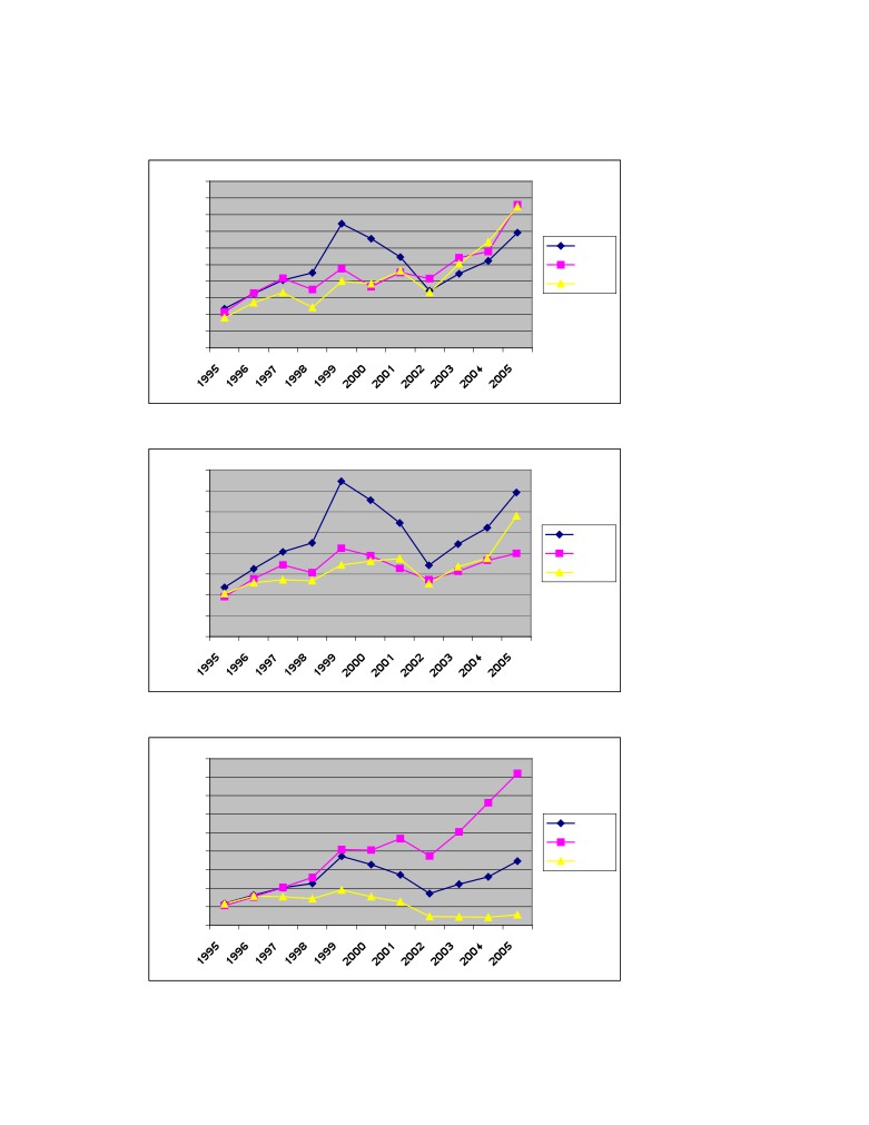
═══════════════════════APPENDIX═══════════════════════

APPENDIX A - Diagrams

500,00

450,00

400,00

350,00

300,00

AFGX

250,00

L-H-H

200,00

L-H-L

150,00

100,00

50,00

0,00

Figure A:1 Total return (buy and hold) from starting value of 100 for L-H-H, L-H-L, AFGX.

400,00

350,00

300,00

250,00

AFGX

200,00

L-M-H

150,00

L-M-L

100,00

50,00

0,00

Figure A:2 Total return from starting value of 100 for L-M-H, L-M-L, AFGX.

900,00

800,00

700,00

600,00

AFGX

500,00

L-L-H

400,00

L-L-L

300,00

200,00

100,00

0,00

Figure A:3 Total return from starting value of 100 for L-L-H, L-L-L, AFGX.

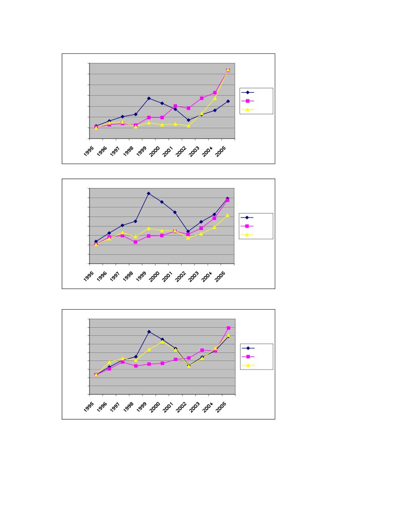
═══════════════════════APPENDIX═══════════════════════

700,00

600,00

500,00

AFGX

400,00

S-H-H

300,00

S-H-L

200,00

100,00

0,00

Figure A:4 Total return from starting value of 100 for S-H-H, S-H-L, AFGX.

400,00

350,00

300,00

250,00

AFGX

200,00

S-M-H

150,00

S-M-L

100,00

50,00

0,00

Figure A:5 Total return from starting value of 100 for S-M-H, S-M-L, AFGX.

450,00

400,00

350,00

300,00

AFGX

250,00

S-L-H

200,00

S-L-L

150,00

100,00

50,00

0,00

Figure A:6 Total return from starting value of 100 for S-L-H, S-L-L, AFGX.

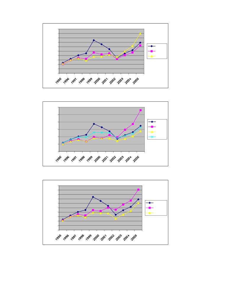
═══════════════════════APPENDIX═══════════════════════

500,00

450,00

400,00

350,00

300,00

AFGX

250,00

Large:

200,00

Small:

150,00

100,00

50,00

0,00

Figure A:7 Total return from starting value of 100 for Large, Small, AFGX.

600,00

500,00

400,00

AFGX

B/P H

300,00

B/P M

200,00

B/P L

100,00

0,00

Figure A:8 Total return from starting value of 100 for B/P High, B/P Medium, B/P Low, AFGX.

500,00

450,00

400,00

350,00

300,00

AFGX

250,00

MOM H

200,00

MOM L

150,00

100,00

50,00

0,00

Figure A:9 Total return from starting value of 100 for Momentum High, Momentum Low, AFGX.

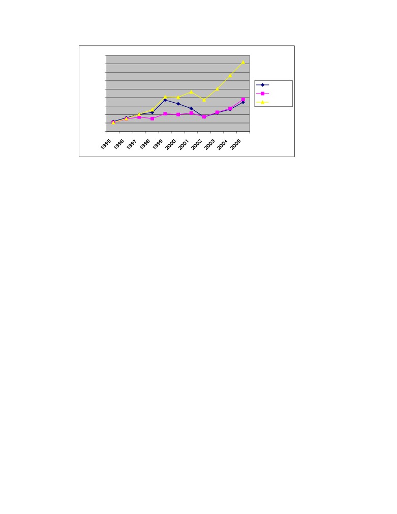
═══════════════════════APPENDIX═══════════════════════

900,00

800,00

700,00

600,00

AFGX

500,00

SMART

400,00

L-L-H

300,00

200,00

100,00

0,00

Figure A:10 Total return from starting value of 100 for SMART (all portfolios), L-L-H and AFGX.

Note: AFGX includes the O-list not only the A-list from 1998 and forward. Total returns is

the same as buy and hold returns discussed in detail in the thesis.

[Back to Accounting Blog]